
20.3: Finite-Difference Equations
- Page ID
- 9661

\( \newcommand{\vecs}[1]{\overset { \scriptstyle \rightharpoonup} {\mathbf{#1}} } \)
\( \newcommand{\vecd}[1]{\overset{-\!-\!\rightharpoonup}{\vphantom{a}\smash {#1}}} \)
\( \newcommand{\dsum}{\displaystyle\sum\limits} \)
\( \newcommand{\dint}{\displaystyle\int\limits} \)
\( \newcommand{\dlim}{\displaystyle\lim\limits} \)
\( \newcommand{\id}{\mathrm{id}}\) \( \newcommand{\Span}{\mathrm{span}}\)
( \newcommand{\kernel}{\mathrm{null}\,}\) \( \newcommand{\range}{\mathrm{range}\,}\)
\( \newcommand{\RealPart}{\mathrm{Re}}\) \( \newcommand{\ImaginaryPart}{\mathrm{Im}}\)
\( \newcommand{\Argument}{\mathrm{Arg}}\) \( \newcommand{\norm}[1]{\| #1 \|}\)
\( \newcommand{\inner}[2]{\langle #1, #2 \rangle}\)
\( \newcommand{\Span}{\mathrm{span}}\)
\( \newcommand{\id}{\mathrm{id}}\)
\( \newcommand{\Span}{\mathrm{span}}\)
\( \newcommand{\kernel}{\mathrm{null}\,}\)
\( \newcommand{\range}{\mathrm{range}\,}\)
\( \newcommand{\RealPart}{\mathrm{Re}}\)
\( \newcommand{\ImaginaryPart}{\mathrm{Im}}\)
\( \newcommand{\Argument}{\mathrm{Arg}}\)
\( \newcommand{\norm}[1]{\| #1 \|}\)
\( \newcommand{\inner}[2]{\langle #1, #2 \rangle}\)
\( \newcommand{\Span}{\mathrm{span}}\) \( \newcommand{\AA}{\unicode[.8,0]{x212B}}\)
\( \newcommand{\vectorA}[1]{\vec{#1}} % arrow\)
\( \newcommand{\vectorAt}[1]{\vec{\text{#1}}} % arrow\)
\( \newcommand{\vectorB}[1]{\overset { \scriptstyle \rightharpoonup} {\mathbf{#1}} } \)
\( \newcommand{\vectorC}[1]{\textbf{#1}} \)
\( \newcommand{\vectorD}[1]{\overrightarrow{#1}} \)
\( \newcommand{\vectorDt}[1]{\overrightarrow{\text{#1}}} \)
\( \newcommand{\vectE}[1]{\overset{-\!-\!\rightharpoonup}{\vphantom{a}\smash{\mathbf {#1}}}} \)
\( \newcommand{\vecs}[1]{\overset { \scriptstyle \rightharpoonup} {\mathbf{#1}} } \)
\(\newcommand{\longvect}{\overrightarrow}\)
\( \newcommand{\vecd}[1]{\overset{-\!-\!\rightharpoonup}{\vphantom{a}\smash {#1}}} \)
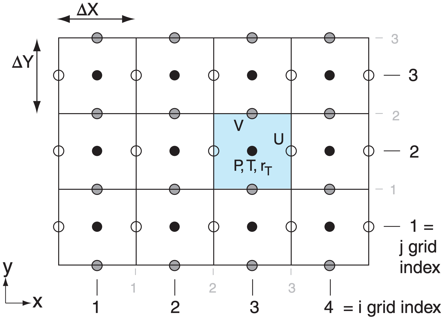
\(\newcommand{\avec}{\mathbf a}\) \(\newcommand{\bvec}{\mathbf b}\) \(\newcommand{\cvec}{\mathbf c}\) \(\newcommand{\dvec}{\mathbf d}\) \(\newcommand{\dtil}{\widetilde{\mathbf d}}\) \(\newcommand{\evec}{\mathbf e}\) \(\newcommand{\fvec}{\mathbf f}\) \(\newcommand{\nvec}{\mathbf n}\) \(\newcommand{\pvec}{\mathbf p}\) \(\newcommand{\qvec}{\mathbf q}\) \(\newcommand{\svec}{\mathbf s}\) \(\newcommand{\tvec}{\mathbf t}\) \(\newcommand{\uvec}{\mathbf u}\) \(\newcommand{\vvec}{\mathbf v}\) \(\newcommand{\wvec}{\mathbf w}\) \(\newcommand{\xvec}{\mathbf x}\) \(\newcommand{\yvec}{\mathbf y}\) \(\newcommand{\zvec}{\mathbf z}\) \(\newcommand{\rvec}{\mathbf r}\) \(\newcommand{\mvec}{\mathbf m}\) \(\newcommand{\zerovec}{\mathbf 0}\) \(\newcommand{\onevec}{\mathbf 1}\) \(\newcommand{\real}{\mathbb R}\) \(\newcommand{\twovec}[2]{\left[\begin{array}{r}#1 \\ #2 \end{array}\right]}\) \(\newcommand{\ctwovec}[2]{\left[\begin{array}{c}#1 \\ #2 \end{array}\right]}\) \(\newcommand{\threevec}[3]{\left[\begin{array}{r}#1 \\ #2 \\ #3 \end{array}\right]}\) \(\newcommand{\cthreevec}[3]{\left[\begin{array}{c}#1 \\ #2 \\ #3 \end{array}\right]}\) \(\newcommand{\fourvec}[4]{\left[\begin{array}{r}#1 \\ #2 \\ #3 \\ #4 \end{array}\right]}\) \(\newcommand{\cfourvec}[4]{\left[\begin{array}{c}#1 \\ #2 \\ #3 \\ #4 \end{array}\right]}\) \(\newcommand{\fivevec}[5]{\left[\begin{array}{r}#1 \\ #2 \\ #3 \\ #4 \\ #5 \\ \end{array}\right]}\) \(\newcommand{\cfivevec}[5]{\left[\begin{array}{c}#1 \\ #2 \\ #3 \\ #4 \\ #5 \\ \end{array}\right]}\) \(\newcommand{\mattwo}[4]{\left[\begin{array}{rr}#1 \amp #2 \\ #3 \amp #4 \\ \end{array}\right]}\) \(\newcommand{\laspan}[1]{\text{Span}\{#1\}}\) \(\newcommand{\bcal}{\cal B}\) \(\newcommand{\ccal}{\cal C}\) \(\newcommand{\scal}{\cal S}\) \(\newcommand{\wcal}{\cal W}\) \(\newcommand{\ecal}{\cal E}\) \(\newcommand{\coords}[2]{\left\{#1\right\}_{#2}}\) \(\newcommand{\gray}[1]{\color{gray}{#1}}\) \(\newcommand{\lgray}[1]{\color{lightgray}{#1}}\) \(\newcommand{\rank}{\operatorname{rank}}\) \(\newcommand{\row}{\text{Row}}\) \(\newcommand{\col}{\text{Col}}\) \(\renewcommand{\row}{\text{Row}}\) \(\newcommand{\nul}{\text{Nul}}\) \(\newcommand{\var}{\text{Var}}\) \(\newcommand{\corr}{\text{corr}}\) \(\newcommand{\len}[1]{\left|#1\right|}\) \(\newcommand{\bbar}{\overline{\bvec}}\) \(\newcommand{\bhat}{\widehat{\bvec}}\) \(\newcommand{\bperp}{\bvec^\perp}\) \(\newcommand{\xhat}{\widehat{\xvec}}\) \(\newcommand{\vhat}{\widehat{\vvec}}\) \(\newcommand{\uhat}{\widehat{\uvec}}\) \(\newcommand{\what}{\widehat{\wvec}}\) \(\newcommand{\Sighat}{\widehat{\Sigma}}\) \(\newcommand{\lt}{<}\) \(\newcommand{\gt}{>}\) \(\newcommand{\amp}{&}\) \(\definecolor{fillinmathshade}{gray}{0.9}\)Here we see how to find discrete numerical approximations to the equations of motion (20.1 - 20.7) as applied to grid cells.
20.3.1. Notation
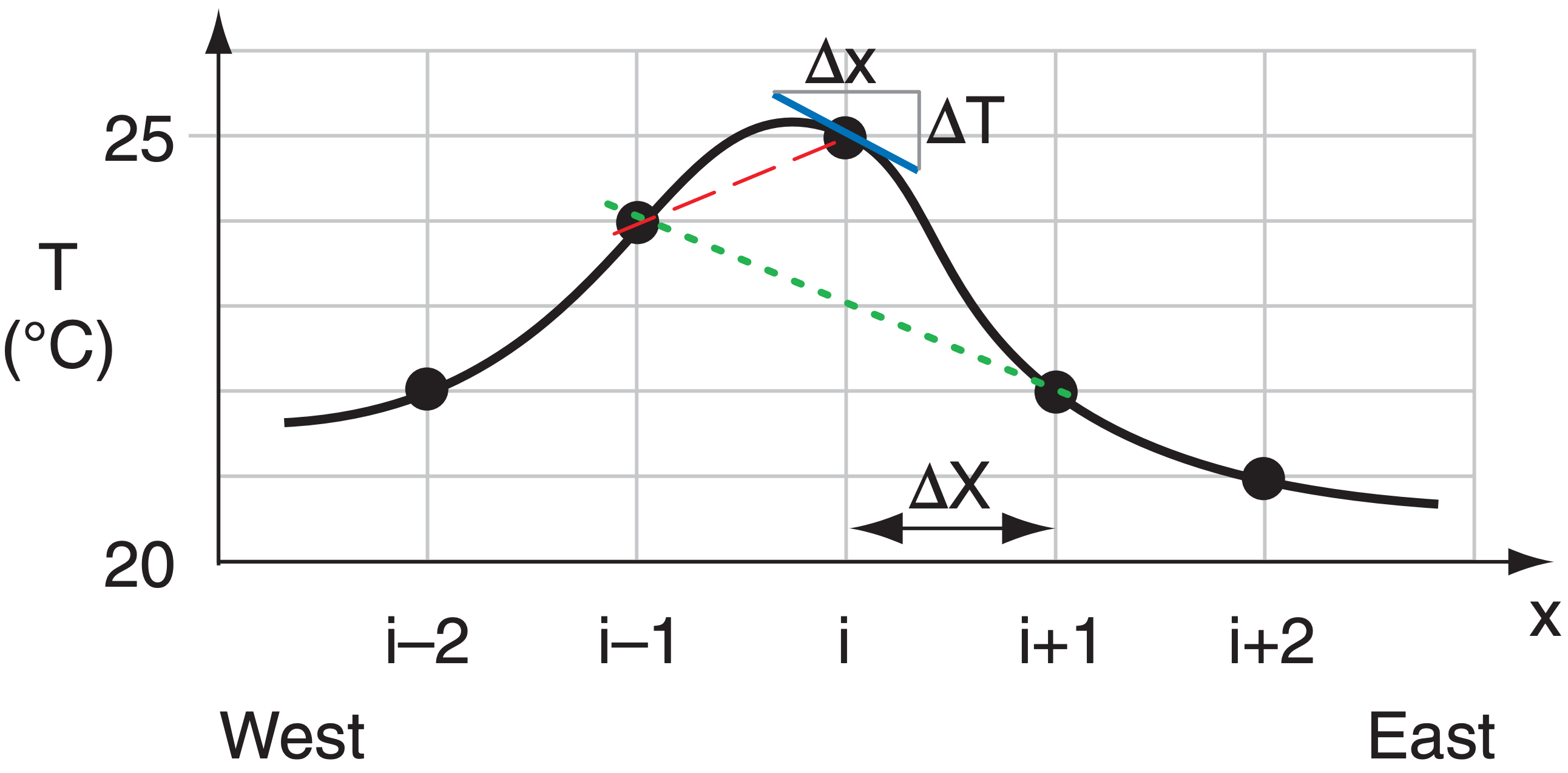
Throughout this book, we have used ratios of differences (such as ∆T/∆x) instead of derivatives (∂T/∂x) to represent the local slope or local gradient of a variable. While this allowed us to avoid calculus, it causes problems in this chapter because ∆x now has two conflicting meanings: (1) ∆x is an infinitesimal increment of distance, such as used to find the local slope of a curve at point i in Fig. 20.8. (2) ∆X is a finite distance between grid points, such as between points i and i+1 in Fig. 20.8.
To artificially discriminate between these two meanings, we will use lower-case “x” in ∆x to represent an infinitesimal distance increment, and upper-case “X” in ∆X to represent a finite distance between grid points.]
20.3.2. Approximations to Spatial Gradients
The equations of motion (20.1 - 20.6) contain many terms involving local gradients, such as the horizontal temperature gradient ∆T/∆x. So to solve these equations, we need a way to approximate the local gradients as a function of things that we know — e.g., values of T at the discrete grid points.
But when the local gradient of an analytical variable is represented at one grid point as a function of its values at other grid points, the result is an infinite sum of terms — each term of greater power of ∆X or ∆t. This is a Taylor series (see the HIGHER MATH box). The most important terms in the series are the first ones — the ones of lowest power of ∆X (said to be of lowest order).
However, the higher-order terms do slightly improve the accuracy. For practical reasons, the numerical forecast can consider only the first few terms from the Taylor series. Such a series is said to be truncated; namely, the highest-order terms are cut from the calculation. For example, a secondorder approximation to T’ (= ∆T/∆x) has an error of about ±T’/6, while a third-order approximation has an error of about ±T’/24.
Different approximations to the local gradients have different truncation errors. Such approximations can be applied to the local gradient of any weather variable — the illustrations below focus on temperature (T) gradients. Assuming a mean wind from the west, an upwind first-order difference approximation is:
\begin{align}\left.\dfrac{\Delta T}{\Delta x}\right|_{i} \approx \dfrac{\left(T_{i}-T_{i-1}\right)}{\Delta X}\tag{20.9}\end{align}
which applies at grid point i. But first-order approximations to the gradient (shown by slope of the dashed line in Fig. 20.8) can have large errors relative to the actual gradient (shown by the slope of the thin black line).
A centered second-order difference gives a better approximation to the gradient at i:
\begin{align}\left.\dfrac{\Delta T}{\Delta x}\right|_{i} \approx \dfrac{\left(T_{i+1}-T_{i-1}\right)}{2 \Delta X}\tag{20.10}\end{align}
as sketched by the dotted line in Fig. 20.8.
An even better centered fourth-order difference for the gradient at i is:
\begin{align}\left.\dfrac{\Delta T}{\Delta x}\right|_{i} \approx \dfrac{1}{12 \Delta X}\left[8\left(T_{i+1}-T_{i-1}\right)-\left(T_{i+2}-T_{i-2}\right)\right]\tag{20.11}\end{align}
as shown by the thin solid line in Fig. 20.8.
Use similar equations for gradients of other variables (U, V, W, rT, ρ). Orders higher than fourth-order are also used in some numerical models.
Sample Application
Find ∆T/∆x at grid point i in Fig. 20.8 using 1, 2, & 4th order gradients, for a horizontal grid spacing of 5 km.
Find the Answer
Given: Ti–2 = 22, Ti–1 = 24, Ti = 25, Ti+1 = 22, Ti+2 = 21°C from the data points in Fig. 20.8. ∆X = 5 km.
Find: ∆T/∆x = ? °C km–1
For Upwind 1st-order Difference, use eq. (20.9):
∆T/∆x ≈ (25 – 24°C)/(5 km) = 0.2 °C km–1
For Centered 2nd-order Difference, use eq. (20.10):
∆T/∆x ≈ (22 – 24°C) /[2·(5 km)] = –0.2 °C km–1
For Centered 4th-order Difference, use eq. (20.11):
∆T/∆x ≈ [8·(22–24°C) – (21–22°C)]/[12·(5 km)] ≈ [ (–16 + 1)°C] /(60 km) = –0.25 °C km–1
Check: Units OK. Agrees with lines in Fig. 20.8.
Exposition: Higher-order differences are better approximations, but none give the true slope exactly
The equations of motion have terms such as U·∂T/∂x. You can use a Taylor series to approximate the derivative ∂T/∂x as a function of discrete gridpoint values. [We will use Lagrange’s notation for derivatives: T’ for ∂T/∂x, and T’’ for ∂2T/∂x2, etc.]
Any analytic function such as temperature vs. distance T(x) can be expanded into an infinite series called a Taylor series if the derivatives (T’, T’’, etc.) are well behaved near x. To find the value of T at (x + ∆X), where ∆X is a small finite distance from x, use a Taylor series of the form:
\begin{align}T(x+\Delta X) \approx T(x)+\dfrac{(\Delta X)^{1}}{1 !} \cdot T^{\prime}(x)+\dfrac{(\Delta X)^{2}}{2 !} \cdot T^{\prime \prime}(x)
+\dfrac{(\Delta X)^{3}}{3 !} \cdot T^{\prime \prime \prime}(x)+\dfrac{(\Delta X)^{4}}{4 !} \cdot T^{\prime \prime \prime \prime}(x)+\ldots]\tag{20.BA1}\end{align}
Apply the Taylor series to grid points (Fig. 20.8), where the spatial position is indicated by an index i:
\begin{align}T_{i+1} \approx T_{i}+\Delta X \cdot T_{i}^{\prime}+\dfrac{(\Delta X)^{2}}{2} \cdot T_{i}^{\prime \prime}+\dfrac{(\Delta X)^{3}}{6} \cdot T_{i}^{\prime \prime \prime}+\dfrac{(\Delta X)^{4}}{24} \cdot T_{i}^{\prime \prime \prime \prime}+\ldots\tag{20.BA2}\end{align}
Similarly, by using –∆X in the Taylor expansion, you can estimate T upwind, at grid index i–1:
\begin{align}T_{i-1} \approx T_{i}-\Delta X \cdot T_{i}^{\prime}+\dfrac{(\Delta X)^{2}}{2} \cdot T_{i}^{\prime \prime}-\dfrac{(\Delta X)^{3}}{6} \cdot T_{i}^{\prime \prime \prime}+\dfrac{(\Delta X)^{4}}{24} \cdot T_{i}^{\prime \prime \prime \prime}-\ldots\tag{20.BA3}\end{align}
For practical reasons, you can truncate the series to a finite number of terms. The more terms you keep, the smaller the truncation error. The lowest power of the ∆X term not used defines the order of the truncation. Higher-order truncations have less error.
• For a simple upwind difference (with poor, firstorder error in ∆X), solve eq (20.BA3) for T’:
\begin{align}T_{i}^{\prime}=\dfrac{\left(T_{i}-T_{i-1}\right)}{\Delta X}+O(\Delta X)\tag{20.BA4}\end{align}
where the last term indicates the truncation error. This T’ value gives the dashed-line slope in Fig. 20.8.
• For a centered difference (with moderate, secondorder error in ∆X), subtract eq. (20.BA3) from (20.BA2) and solve the result for T’:
\begin{align}T_{i}^{\prime}=\dfrac{\left(T_{i+1}-T_{i-1}\right)}{2 \Delta X}+O(\Delta X)^{2}\tag{20.BA5}\end{align}
This T’ value gives the dotted-line slope in Fig. 20.8.
For an even better 4th-order centered difference, use:
\begin{align}T_{i}^{\prime}=\dfrac{1}{12 \Delta X}\left[8\left(T_{i+1}-T_{i-1}\right)-\left(T_{i+2}-T_{i-2}\right)\right]+O(\Delta X)^{4}\tag{20.BA6}\end{align}
which is a slightly better fit to the true slope at i.
In this chapter, we use ∆T/∆x in place of T’. Hence, the bullets above give approximations to ∆T/∆x.
20.3.3. Grid Computation Rules
(1) When multiplying or dividing any two variables, both of those variables must be at the same point in space. The result applies at that same point.
(2) When adding, averaging, or subtracting any two variables, if both those variables are at the same point in space, then the result applies at the same point.
(3) However, when adding, averaging, or subtracting two variables at different locations in space, the sum, average, or difference applies at a physical location halfway between the locations of the original variables.
For mathematical and physical consistency, the grid computation rules at left must be obeyed when making calculations with grid-point values. Rule 3 is handy because you can use it to “move” values to locations where you can then multiply by other variables while obeying Rule 1.
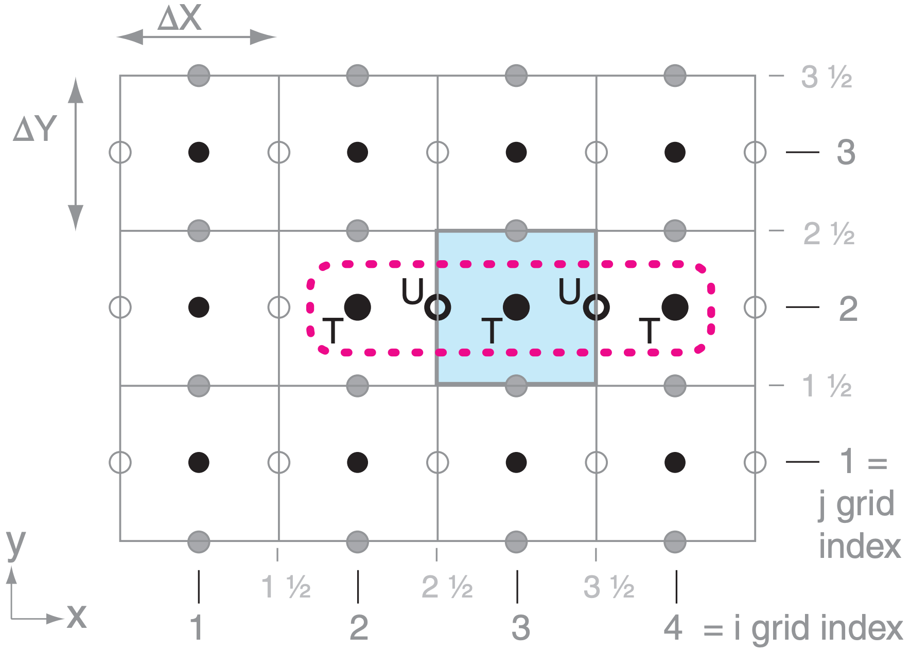
For example, consider the temperature forecast equation (20.4) for grid point (i = 3, j = 2), for the Cgrid in Fig. 20.9. The first term on the right side of eq. (20.4) is temperature advection in the x-direction. If we choose to use second-order difference eq. (20.10) at location (i,j) = (3,2), we have a mismatch because we do not have wind at that same location. Rule 1 says we can not multiply the wind times the T gradient.
However, we can use Rule 3 to average the Uwinds from the right and left of the temperature point, knowing that this average applies halfway between the two U points. The average thus spatially coincides with the temperature gradient, so we can multiply the two factors together.
For that one grid point (i,j) = (3,2), the result is:
\begin{align}\left\{-U \cdot \dfrac{\Delta T}{\Delta x}\right\}_{3,2} \approx-\left(\dfrac{U_{3\ 1 /_ 2,2}+U_{2\ 1 / _2,2}}{2}\right) \cdot\left[\dfrac{T_{4,2}-T_{2,2}}{2 \cdot \Delta X}\right]\tag{20.12}\end{align}
where the ½ grid index numbering method was used for values at the edges of the grid cell (Fig. 20.9). The parentheses hold the average U, and the square brackets hold the centered second-order difference approximation for the local T gradient.
Similarly, for any grid point (i,j), the result is:
\begin{align}\left\{-U \cdot \dfrac{\Delta T}{\Delta x}\right\}_{i, j} \approx-\left(\dfrac{U_{i+1/_2,\ j}+U_{i-1 /_2,\ j}}{2}\right) \cdot\left[\dfrac{T_{i+1,\ j}-T_{i-1,\ j}}{2 \cdot \Delta X}\right]\tag{20.13}\end{align}
The spatial arrangement of all grid points used in any calculation is called a stencil. Fig. 20.9 shows the stencil for eq. (20.13). Different grid arrangements (Grids A - E) and different approximation orders will result in different stencils.
Significantly, the forecast for any one grid point (such as i,j) depends on the values at other nearby grid points [such as (i–1,j) , (i–½,j) , (i+½,j) , (i+1,j) ]. In turn, forecasts at each of these points depends on values at their neighbors. This interconnectivity is summarized as NWP Corollary 1, at left.
For grid points near the edges of the domain, special stencils using one-sided difference approximations must be used, to avoid referencing grid points that don’t exist because they are outside of the domain. Alternately, a halo of ghost-cell grid points outside the forecast domain can be specified using values found from a larger coarser domain or from imposed boundary conditions (BCs; i.e., the state of the air along the edges of the forecast domain).
Sample Application
What is the warming rate at grid point (i=3, j=2) in Fig. 20.9 due to temperature advection in the x-direction, given T2,2 = 22°C, T3,2 = 23°C, T4,2 = 24°C, U2½,2 = –5 m s–1, U3½,2 = –7 m s–1, ∆X = 10 km?
Find the Answer
Given: T and U values above. ∆X = 10 km
Find: ∆T/∆t = –U·∆T/∆x = ? °C h–1.
Use eq. (20.12):
∆T/∆t ≈ –0.5·(–7–5 m s–1) · [ 0.5·(24 – 22°C)/(104m) ] ≈ (6 m s–1) · [ 1°C/(104m) ] · (3600 s h–1) = 2.16 °C h–1.
Check: Units OK. Sign OK. Magnitude OK.
Exposition: Winds are advecting in warmer air from the East, causing advective warming.
NWP Corollary 1: The forecast at any one point is affected by ALL other points in the forecast domain.
20.3.4. Time Differencing
The smooth flow of time implied by the left side of the equations of motion can be approximated by a sequence of discrete time steps, each of duration ∆t. For example, the temperature tendency term on the left side of eq. (20.4) can be written as a centered time difference:
\begin{align}\dfrac{\Delta T}{\Delta t} \approx \dfrac{T(t+\Delta t)-T(t-\Delta t)}{2 \cdot \Delta t}\tag{20.14}\end{align}
When combined with the right side of eq. (20.4), the result gives the temperature at some future time as a function of the temperatures and winds at earlier times:
\begin{align}T_{3,2}(t+\Delta t)=T_{3,2}(t-\Delta t)+2 \Delta t \cdot[\mathrm{RHS} \text { of eq. } 20.4]\tag{20.15}\end{align}
Typical time-step durations ∆t are on the order of a few seconds to tens of minutes, depending on the grid size (see the section on numerical stability).
The equation above is a form of the leapfrog scheme (Fig. 20.10). It gets its name because the forecast starts from the previous time step (t–∆t) and leaps over the present step (t) to make a forecast for the future (t+∆t). Although it leaps over the present step, it utilizes the present conditions to determine the future conditions (e.g., eq. 20.16 below).
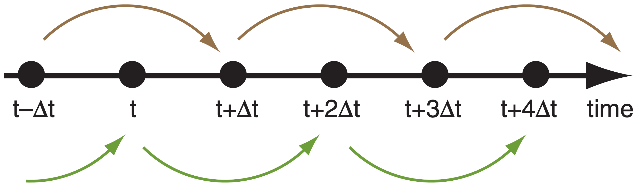
The two leapfrog solutions (one starting at t–∆t and the other starting at t, illustrated above and below the timeline in Fig. 20.10) sometimes diverge from each other, and need to be occasionally averaged together to yield a consistent forecast. Without such averaging the solution would become unstable, and would numerically blow up (see next section).
There are other numerical solutions that work better than the leapfrog method. One example is the Runge-Kutta method, described in the INFO Box.
By combining eqs. (20.12 & 20.15), we get a temperature forecast equation that includes only the Uadvection forcing:
\begin{align}T_{3,2}(t+\Delta t) =T_{3,2}(t-\Delta t)+
\dfrac{\Delta t}{\Delta X} \cdot\left\{\left(U_{3\ 1/_2,2}+U_{2\ 1/_2,2}\right) \cdot 1 / 2\left[T_{4,2}-T_{2,2}\right]\right\}_{t}\tag{20.16}\end{align}
where the subscript t at the very right indicates that all of the terms inside the curly brackets are evaluated at time t. So the future temperature (at t+∆t), depends on the current temperature and winds (at t) and on the past temperature (at t–∆t). The concept of a stencil can be extended to include the 4-D arrangement of locations and times needed to forecast one aspect of physics for any grid point.
Generalizing the previous equation, and recalling NWP Corollary 1, we infer that: the forecast ∆t into the future of any one variable at one location can depend on the current state of ALL other variables at ALL other locations. Thus, ALL other variable at ALL other locations must be stepped forward the same one ∆t into the future, based on current values. Only after they all have made this step can we proceed to the next step, to get to time t + 2∆t into the future. This characteristic is summarized as NWP Corollary 2:
NWP Corollary 2: ALL variables at ALL grid points must march in step into the future*.
*Some terms (e.g., for acoustic waves) and some parameterizations require very short time steps for numerical stability. They can be programmed to take many “baby” steps for each “adult” time step ∆t in the model, to enable them to remain synchronized (holding hands) as they advance toward the future.
To start the whole NWP, we need initial conditions (ICs). These ICs are estimated by merging weather observations with past forecasts (see the Data Assimilation section). ICs are often named by the synoptic time when most of the observations were made, such as the “00 UTC analysis”, the “00 UTC initialization”, or the “00 UTC model run”. Modern assimilation schemes can also incorporate asynoptic (off-hour) observations.
The prognostic equations of motion (20.1 - 20.6) can be written in a generic form:
\(\ \Delta A / \Delta t=f[A, x, t]\)
where A is any dependent variable (e.g., U, V, W, T, etc.), f is a function that describes all the dynamics and physics of the equations of motion, and x represents all other independent variables (x, y, z) as indicated by grid-point indices (i, j, k). Knowing present (at time t) and all past values at the grid points, how do we make a small time step ∆t into the future?
One of the simplest methods is called the Euler method (also known as the Euler-forward method):
\(\ A(t+\Delta t)=A(t)+\Delta t \cdot f[A(t), x, t]\)
But this is only first-order accurate, and is never used because errors accumulate so quickly that the numerical forecast often blows up (forecasts values of ± infinity) causing the computer to crash (premature termination due to computation errors).
The leapfrog method was described in the text, and is second-order accurate.
\(\ A(t+\Delta t)=A(t-\Delta t)+2 \Delta t \cdot f[A(t), x, t]\)
Higher-order accuracy has less error.
Also popular is the fourth-order Runge-Kut- ta method, which has even less error, but requires intermediate steps done in the order listed:
(1) k1 = f[ A(t) , x , t ]
(2) k2 = f[ A(t)+½∆t·k1, x , t+½∆t ]
(3) k3 = f[ A(t)+½∆t·k2 , x , t+½∆t ]
(4) k4 = f[ A(t)+∆t·k3 , x , t+∆t ]
(5) A(t+∆t) = A(t) + (∆t/6)·[ k1 + 2k2 + 2k3 + k4 ]
Sample Application (§)
Given a 1-D array consisting of 10 grid points in the xdirection with the following initial temperatures (°C): Ti (t = 0) = 21.76 22.85 22.85 21.76 20.00 18.24 17.15 17.15 18.24 20.00 for i = 1 to 10.
Assume that the lateral boundaries are cyclic, so that this number sequence repeats outside this primary domain. Grid spacing is 3 km and wind speed from the west is 10 m s–1. For a 250 s time step, forecast the temperature at each point for the first 6 time steps, using leapfrog temporal and 4th-order centered spatial differences.
Find the Answer
Given: ∆X = 3 km , ∆t = 250 s , U = 10 m s–1. Initially:
| i = | 1 | 2 | 3 | 4 | 5 | 6 | 7 | 8 | 9 | 10 |
| T = | 21.76 | 22.85 | 22.85 | 21.76 | 20.00 | 18.24 | 17.15 | 17.15 | 18.24 | 20.00 |
Find: Ti at t = 250 s, 500 s, etc. out to 1500 s
We can use leapfrog for every time step except the first step, because for the first step we have no temperatures before time zero. So I will use an Eulerian time difference for the first step. The resulting eqs. are:
For 1st time step:
\(\ T_{i}(t+\Delta t)=T_{i}(t=0)-\dfrac{\Delta t \cdot U}{\Delta X \cdot 12}\left[8 \cdot\left(T_{i+1}-T_{i-1}\right)-\left(T_{i+2}-T_{i-2}\right)\right]_{t=0}\)
For all other time steps:
\(\ T_{i}(t+\Delta t)=T_{i}(t-\Delta t)-\dfrac{\Delta t \cdot U \cdot 2}{\Delta X \cdot 12}\left[8 \cdot\left(T_{i+1}-T_{i-1}\right)-\left(T_{i+2}-T_{i-2}\right)\right]_{t}\)
Solving these in a spreadsheet gives, the following, where each row is a new time step and each column is a different grid point:
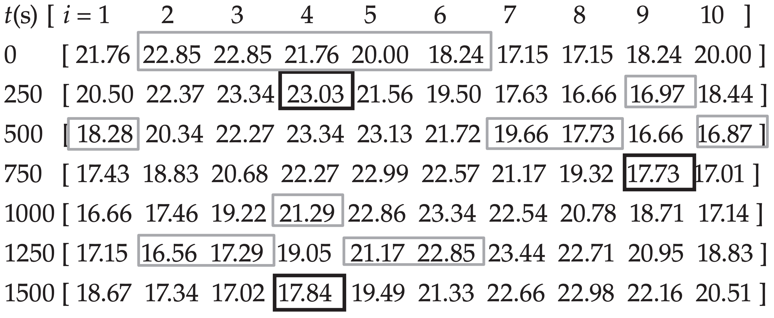
These are plotted as Fig. 20.11b, showing a temperature pattern that is advected by the wind toward the East.
Check: Units OK. Fig. 20.11b looks reasonable
Exposition: The Courant Number [∆t·U/∆x] is (250 s) · (10 m s–1) / (3000 m) = 0.833 (dimensionless). Since this number is less than 1, it says that the solution could be numerically stable (see the Numerical Error section).
The boxes in the table above show which numbers are used in the calculation. For example, the temperature forecast at i = 4 and t = 1500 s used data from the grey boxes near it, based on leapfrog in time and 4thorder centered in space. For i = 4 and t = 250 s, the Euler forward time difference was used. For i = 9 and t = 750 s, one of the grey boxes wrapped around, due to the cyclic boundary conditions.
20.3.5. Discretized Equations of Motion
In summary, the physical equations of motion, which are essentially smooth analytical functions, must be discretized to work at grid points. For example, if we use leapfrog time differencing with second-order spatial differencing on a C-grid, the temperature forecast equation (20.4) becomes:
\begin{align}T_{i, j, k}(t+\Delta t)=T_{i, j, k}(t-\Delta t)+2 \Delta t \cdot\{
-\left(\dfrac{U_{i+1 / 2}, j, k+U_{i-1 / 2}, j, k}{2}\right) \cdot\left[\dfrac{T_{i+1, j, k}-T_{i-1, j, k}}{2 \cdot \Delta X}\right]
-\left(\dfrac{V_{i, j+1 / 2, k}+V_{i, j-1 / 2, k}}{2}\right) \cdot\left[\dfrac{T_{i, j+1, k}-T_{i, j-1, k}}{2 \cdot \Delta Y}\right]
-\left(\dfrac{W_{i, j, k+1 / 2}+W_{i, j, k-1 / 2}}{2}\right) \cdot\left[\dfrac{T_{i, j, k+1}-T_{i, j, k-1}}{2 \cdot \Delta Z}\right]
-\dfrac{\mathfrak{R} \cdot T_{i, j, k}}{P_{i, j, k} \cdot C_{p}} \cdot\left[\dfrac{\mathbb{F}_{z\ rad\ i,\ j,\ k+1 / 2}-\mathbb{F}_{z\ r a d\ i,\ j,\ k-1 / 2}}{\Delta Z}\right]
\quad+\dfrac{L_{v}}{C_{p}} \cdot\left[\dfrac{r_{\text {cond }} i, j, k(t+\Delta t)-r_{\text {cond } i, j, k}(t-\Delta t)}{2 \Delta t}\right]
-\left[\dfrac{F_{z\ turb\ i, j, k+1 / 2} -F_{z\ turb\ i,\ j,\ k-1/2}}{\Delta Z}\right]\tag{20.17}\}\end{align}
Finite-difference equations that are used to forecast winds and humidity are similar. If we had used higher-order differencing, and included the curvature terms and mapping factors, the result would have contained even more terms.
Although the equation above looks complicated, it is trivial for a digital computer to solve because it is just algebra. Computing this equation takes a finite time — perhaps a few microseconds. Similar computation time must be spent for all the other grid points in the domain. These computations must be repeated for a succession of short time steps to reach forecast durations of several days. Thus, for many grid points and many time steps, the total computer run-time accumulates and can take many minutes to several hours on powerful computers.