13.4: Spin-up of Cyclonic Rotation
- Page ID
- 9613

\( \newcommand{\vecs}[1]{\overset { \scriptstyle \rightharpoonup} {\mathbf{#1}} } \)
\( \newcommand{\vecd}[1]{\overset{-\!-\!\rightharpoonup}{\vphantom{a}\smash {#1}}} \)
\( \newcommand{\dsum}{\displaystyle\sum\limits} \)
\( \newcommand{\dint}{\displaystyle\int\limits} \)
\( \newcommand{\dlim}{\displaystyle\lim\limits} \)
\( \newcommand{\id}{\mathrm{id}}\) \( \newcommand{\Span}{\mathrm{span}}\)
( \newcommand{\kernel}{\mathrm{null}\,}\) \( \newcommand{\range}{\mathrm{range}\,}\)
\( \newcommand{\RealPart}{\mathrm{Re}}\) \( \newcommand{\ImaginaryPart}{\mathrm{Im}}\)
\( \newcommand{\Argument}{\mathrm{Arg}}\) \( \newcommand{\norm}[1]{\| #1 \|}\)
\( \newcommand{\inner}[2]{\langle #1, #2 \rangle}\)
\( \newcommand{\Span}{\mathrm{span}}\)
\( \newcommand{\id}{\mathrm{id}}\)
\( \newcommand{\Span}{\mathrm{span}}\)
\( \newcommand{\kernel}{\mathrm{null}\,}\)
\( \newcommand{\range}{\mathrm{range}\,}\)
\( \newcommand{\RealPart}{\mathrm{Re}}\)
\( \newcommand{\ImaginaryPart}{\mathrm{Im}}\)
\( \newcommand{\Argument}{\mathrm{Arg}}\)
\( \newcommand{\norm}[1]{\| #1 \|}\)
\( \newcommand{\inner}[2]{\langle #1, #2 \rangle}\)
\( \newcommand{\Span}{\mathrm{span}}\) \( \newcommand{\AA}{\unicode[.8,0]{x212B}}\)
\( \newcommand{\vectorA}[1]{\vec{#1}} % arrow\)
\( \newcommand{\vectorAt}[1]{\vec{\text{#1}}} % arrow\)
\( \newcommand{\vectorB}[1]{\overset { \scriptstyle \rightharpoonup} {\mathbf{#1}} } \)
\( \newcommand{\vectorC}[1]{\textbf{#1}} \)
\( \newcommand{\vectorD}[1]{\overrightarrow{#1}} \)
\( \newcommand{\vectorDt}[1]{\overrightarrow{\text{#1}}} \)
\( \newcommand{\vectE}[1]{\overset{-\!-\!\rightharpoonup}{\vphantom{a}\smash{\mathbf {#1}}}} \)
\( \newcommand{\vecs}[1]{\overset { \scriptstyle \rightharpoonup} {\mathbf{#1}} } \)
\(\newcommand{\longvect}{\overrightarrow}\)
\( \newcommand{\vecd}[1]{\overset{-\!-\!\rightharpoonup}{\vphantom{a}\smash {#1}}} \)
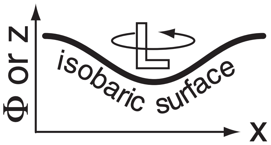
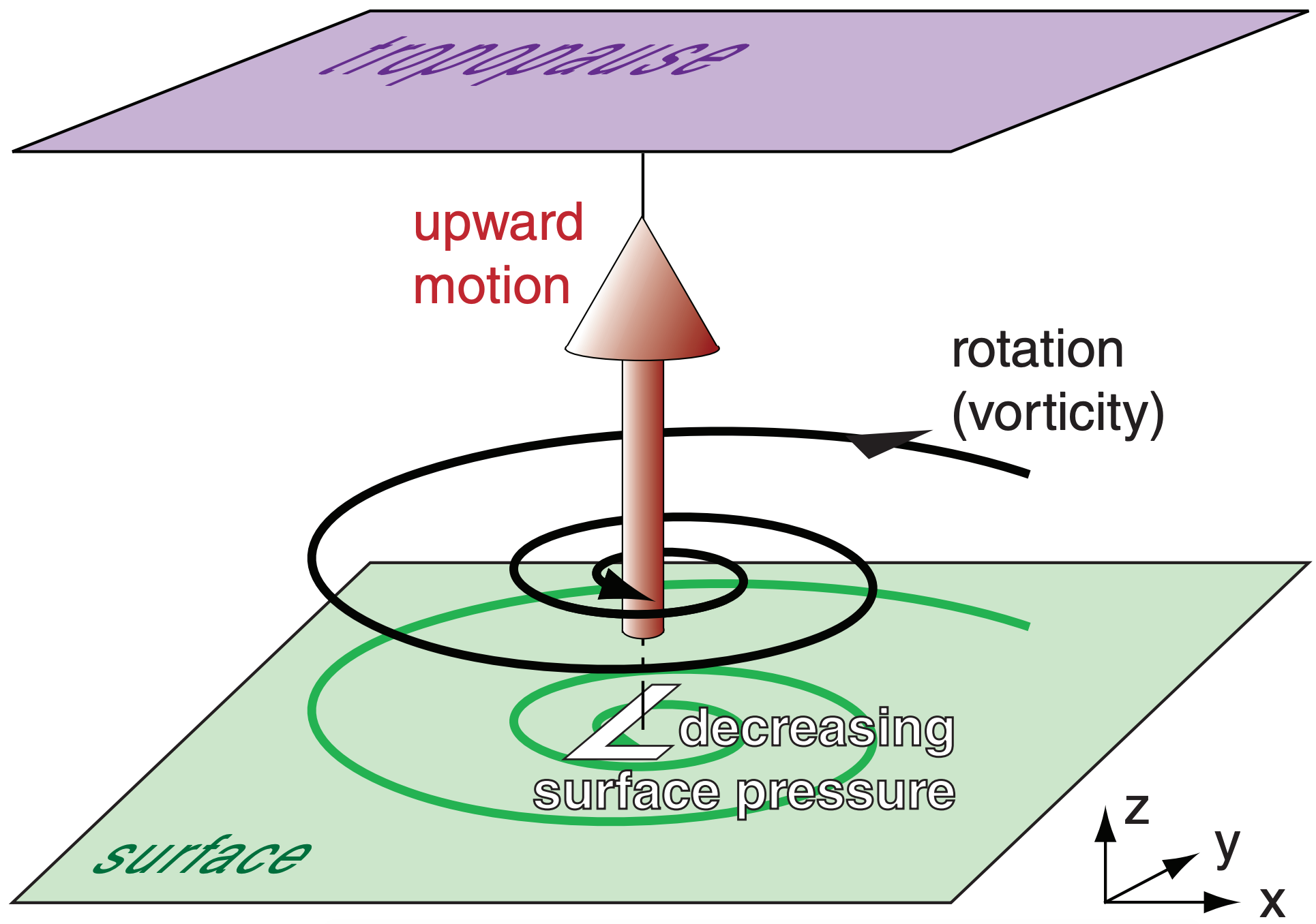
\(\newcommand{\avec}{\mathbf a}\) \(\newcommand{\bvec}{\mathbf b}\) \(\newcommand{\cvec}{\mathbf c}\) \(\newcommand{\dvec}{\mathbf d}\) \(\newcommand{\dtil}{\widetilde{\mathbf d}}\) \(\newcommand{\evec}{\mathbf e}\) \(\newcommand{\fvec}{\mathbf f}\) \(\newcommand{\nvec}{\mathbf n}\) \(\newcommand{\pvec}{\mathbf p}\) \(\newcommand{\qvec}{\mathbf q}\) \(\newcommand{\svec}{\mathbf s}\) \(\newcommand{\tvec}{\mathbf t}\) \(\newcommand{\uvec}{\mathbf u}\) \(\newcommand{\vvec}{\mathbf v}\) \(\newcommand{\wvec}{\mathbf w}\) \(\newcommand{\xvec}{\mathbf x}\) \(\newcommand{\yvec}{\mathbf y}\) \(\newcommand{\zvec}{\mathbf z}\) \(\newcommand{\rvec}{\mathbf r}\) \(\newcommand{\mvec}{\mathbf m}\) \(\newcommand{\zerovec}{\mathbf 0}\) \(\newcommand{\onevec}{\mathbf 1}\) \(\newcommand{\real}{\mathbb R}\) \(\newcommand{\twovec}[2]{\left[\begin{array}{r}#1 \\ #2 \end{array}\right]}\) \(\newcommand{\ctwovec}[2]{\left[\begin{array}{c}#1 \\ #2 \end{array}\right]}\) \(\newcommand{\threevec}[3]{\left[\begin{array}{r}#1 \\ #2 \\ #3 \end{array}\right]}\) \(\newcommand{\cthreevec}[3]{\left[\begin{array}{c}#1 \\ #2 \\ #3 \end{array}\right]}\) \(\newcommand{\fourvec}[4]{\left[\begin{array}{r}#1 \\ #2 \\ #3 \\ #4 \end{array}\right]}\) \(\newcommand{\cfourvec}[4]{\left[\begin{array}{c}#1 \\ #2 \\ #3 \\ #4 \end{array}\right]}\) \(\newcommand{\fivevec}[5]{\left[\begin{array}{r}#1 \\ #2 \\ #3 \\ #4 \\ #5 \\ \end{array}\right]}\) \(\newcommand{\cfivevec}[5]{\left[\begin{array}{c}#1 \\ #2 \\ #3 \\ #4 \\ #5 \\ \end{array}\right]}\) \(\newcommand{\mattwo}[4]{\left[\begin{array}{rr}#1 \amp #2 \\ #3 \amp #4 \\ \end{array}\right]}\) \(\newcommand{\laspan}[1]{\text{Span}\{#1\}}\) \(\newcommand{\bcal}{\cal B}\) \(\newcommand{\ccal}{\cal C}\) \(\newcommand{\scal}{\cal S}\) \(\newcommand{\wcal}{\cal W}\) \(\newcommand{\ecal}{\cal E}\) \(\newcommand{\coords}[2]{\left\{#1\right\}_{#2}}\) \(\newcommand{\gray}[1]{\color{gray}{#1}}\) \(\newcommand{\lgray}[1]{\color{lightgray}{#1}}\) \(\newcommand{\rank}{\operatorname{rank}}\) \(\newcommand{\row}{\text{Row}}\) \(\newcommand{\col}{\text{Col}}\) \(\renewcommand{\row}{\text{Row}}\) \(\newcommand{\nul}{\text{Nul}}\) \(\newcommand{\var}{\text{Var}}\) \(\newcommand{\corr}{\text{corr}}\) \(\newcommand{\len}[1]{\left|#1\right|}\) \(\newcommand{\bbar}{\overline{\bvec}}\) \(\newcommand{\bhat}{\widehat{\bvec}}\) \(\newcommand{\bperp}{\bvec^\perp}\) \(\newcommand{\xhat}{\widehat{\xvec}}\) \(\newcommand{\vhat}{\widehat{\vvec}}\) \(\newcommand{\uhat}{\widehat{\uvec}}\) \(\newcommand{\what}{\widehat{\wvec}}\) \(\newcommand{\Sighat}{\widehat{\Sigma}}\) \(\newcommand{\lt}{<}\) \(\newcommand{\gt}{>}\) \(\newcommand{\amp}{&}\) \(\definecolor{fillinmathshade}{gray}{0.9}\)Cyclogenesis is associated with: (a) upward motion, (b) decreasing surface pressure, and (c) increasing vorticity (i.e., spin-up). You can gain insight into cyclogenesis by studying all three characteristics, even though they are intimately related (Fig. 13.22). Let us start with vorticity.
The equation that forecasts change of vorticity with time is called the vorticity tendency equation. We can investigate the processes that cause cyclogenesis (spin up; positive-vorticity increase) and cyclolysis (spin down; positive-vorticity decrease) by examining terms in the vorticity tendency equation. Mountains are not needed for these processes.
13.4.1. Vorticity Tendency Equation
The change of relative vorticity ζr over time (i.e., the spin-up or vorticity tendency) can be predicted using the following equation:
\(\ \begin{align} \tag{13.9}\end{align}\)
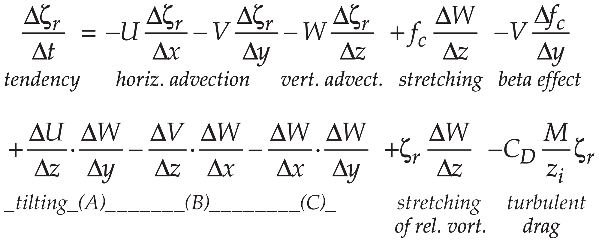
Positive vorticity tendency indicates cyclogenesis.
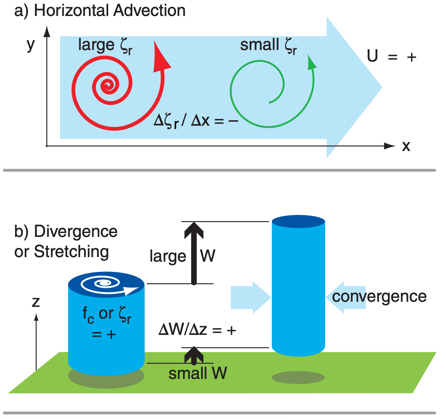
Vorticity Advection: If the wind blows air of greater vorticity into your region of interest, then this is called positive vorticity advection (PVA). Negative vorticity advection (NVA) is when lower-vorticity air is blown into a region. These advections can be caused by vertical winds and horizontal winds (Fig. 13.23a).
Stretching: Consider a short column of air that is spinning as a vortex tube. Horizontal convergence of air toward this tube will cause the tube to become taller and more slender (smaller diameter). The taller or stretched vortex tube supports cyclogenesis (Fig. 13.23b). Conversely, horizontal divergence shortens the vortex tube and supports cyclolysis or anticyclogenesis. In the first and second lines of eq. (13.9) are the stretching terms for Earth’s rotation and relative vorticity, respectively. Stretching means that the top of the vortex tube moves upward away from (or moves faster than) the movement of the bottom of the vortex tube; hence ∆W/∆z is positive for stretching.
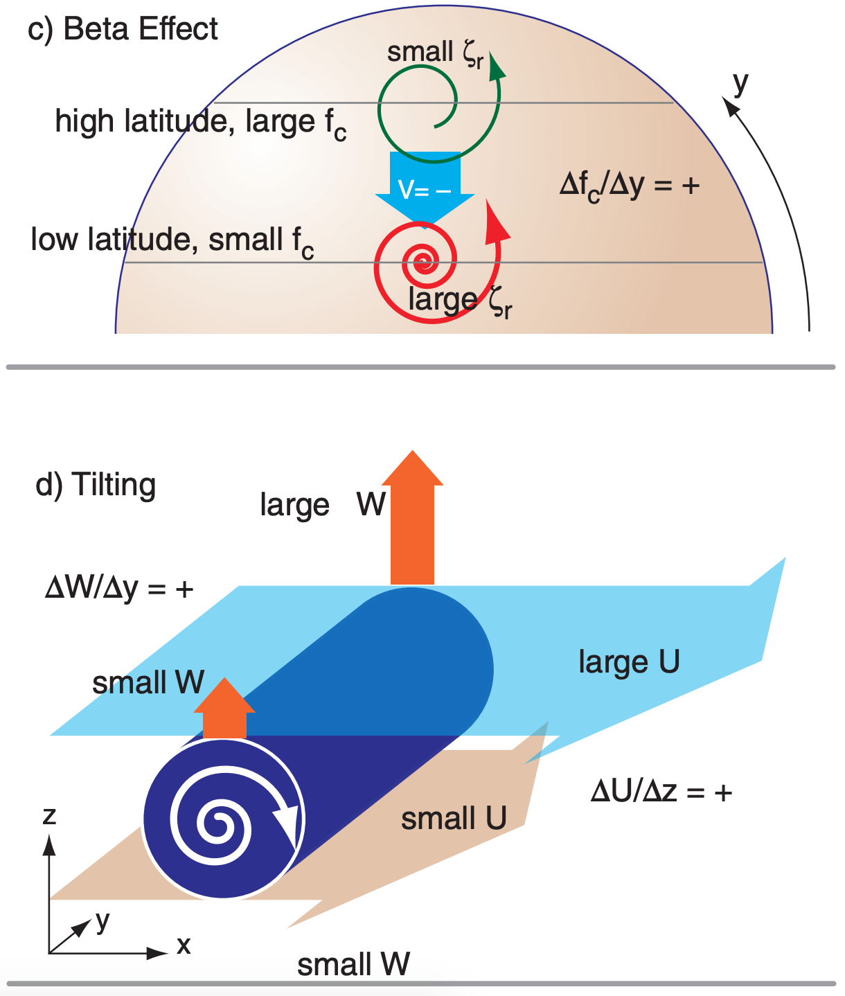
Beta Effect: Recall from eq. (11.35) in the General Circulation chapter that we can define β = ∆fc/∆y. Beta is positive in the N. Hemisphere because the Coriolis parameter increases toward the north pole (see eq. 13.2). If wind moves air southward (i.e., V = negative) to where fc is smaller, then relative vorticity ζr becomes larger (as indicated by the negative sign in front of the beta term) to conserve potential vorticity (Fig. 13.23c).
Tilting Terms: (A & B in eq. 13.9) If the horizontal winds change with altitude, then this shear causes vorticity along a horizontal axis. (C in eq. 13.9) Neighboring up- and down-drafts give horizontal shear of the vertical wind, causing vorticity along a horizontal axis. (A-C) If a resulting horizontal vortex tube experiences stronger vertical velocity on one end relative to the other (Fig. 13.23d), then the tube will tilt to become more vertical. Because spinning about a vertical axis is how we define vorticity, we have increased vorticity via the tilting of initially horizontal vorticity.
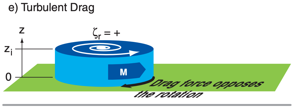
Turbulence in the atmospheric boundary layer (ABL) communicates frictional forces from the ground to the whole ABL. This turbulent drag acts to slow the wind and decrease rotation rates (Fig. 13.23e). Such spin down can cause cyclolysis.
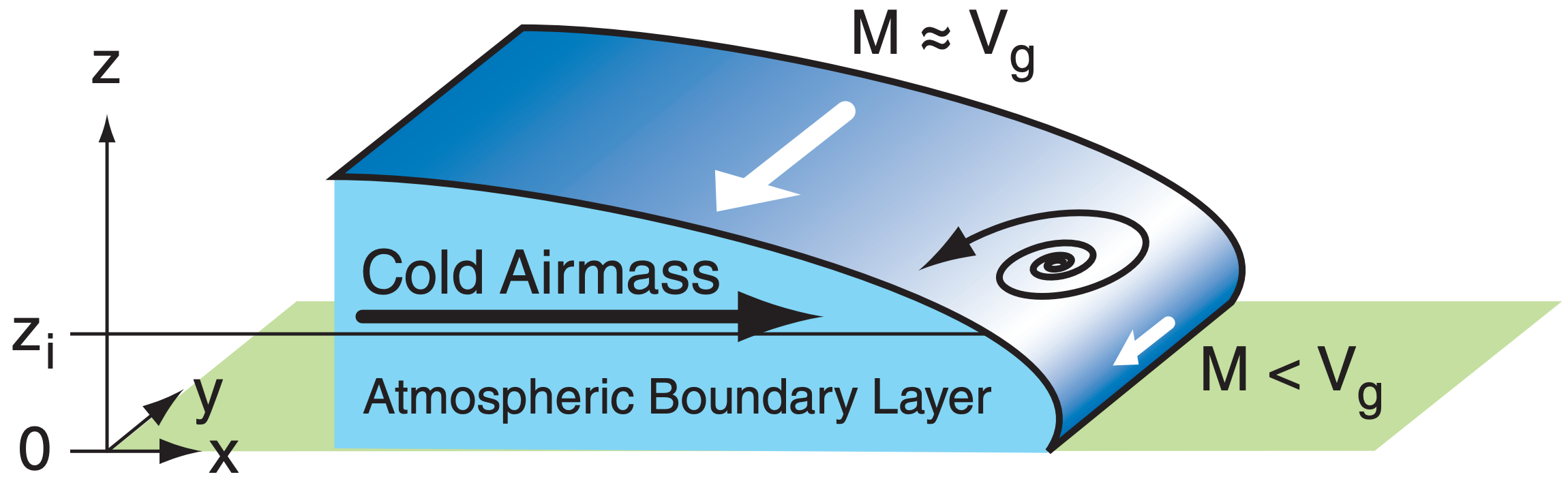
However, for cold fronts drag can increase vorticity. As the cold air advances (black arrow in Fig. 13.23f), Coriolis force will turn the winds and create a geostrophic wind Vg (large white arrow). Closer to the leading edge of the front where the cold air is shallower, the winds M are subgeostrophic because of the greater drag. The result is a change of wind speed M with distance x that causes positive vorticity.
All of the terms in the vorticity-tendency equation must be summed to determine net spin down or spin up. You can identify the action of some of these terms by looking at weather maps.
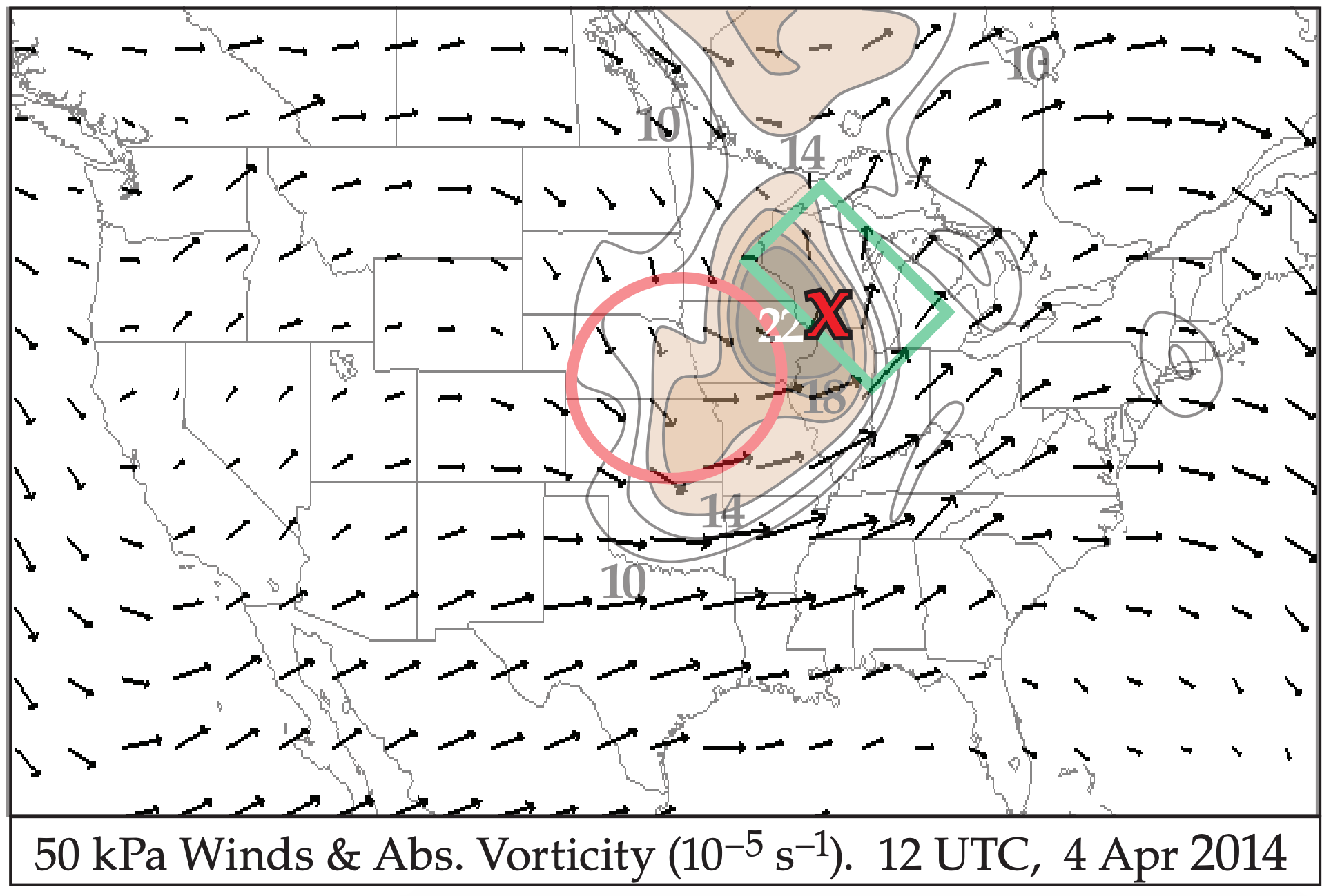
Fig. 13.24 shows the wind vectors and absolute vorticity on the 50 kPa isobaric surface (roughly in the middle of the troposphere) for the case-study cyclone. Positive vorticity advection (PVA) occurs where wind vectors are crossing the vorticity contours from high toward low vorticity, such as highlighted by the dark box in Fig. 13.24. Namely, higher vorticity air is blowing into regions that contained lower vorticity. This region favors cyclone spin up.
Negative vorticity advection (NVA) is where the wind crosses the vorticity contours from low to high vorticity values (dark oval in Fig. 13.24). By using the absolute vorticity instead of relative vorticity, Fig. 13.24 combines the advection and beta terms.
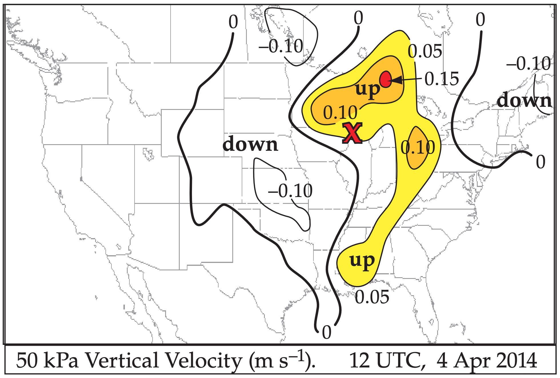
Fig. 13.25 shows vertical velocity in the middle of the atmosphere. Since vertical velocity is near zero at the ground, regions of positive vertical velocity at 50 kPa must correspond to stretching in the bottom half of the atmosphere. Thus, the updraft regions in the figure favor cyclone spin-up (i.e., cyclogenesis).
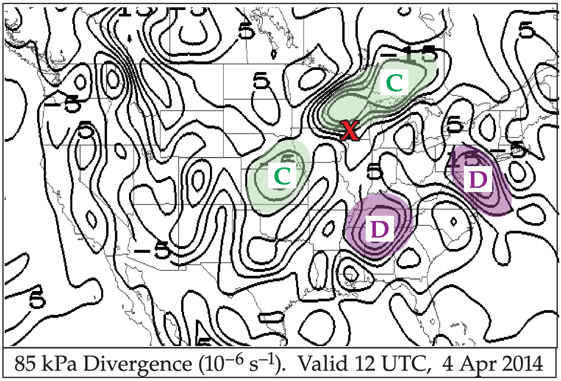
In the bottom half of the troposphere, regions of stretching must correspond to regions of convergence of air, due to mass continuity. Fig. 13.26 shows the divergence field at 85 kPa. Negative divergence corresponds to convergence. The regions of low-altitude convergence favor cyclone spin-up.
Low-altitude spin-down due to turbulent drag occurs wherever there is rotation. Thus, the rotation of 10 m wind vectors around the surface low in Fig. 13.13 indicate vorticity that is spinning down. The tilting term will also be discussed in the Thunderstorm chapters, regarding tornado formation.
13.4.2. Quasi-Geostrophic Approximation
Above the boundary layer (and away from fronts, jets, and thunderstorms) the terms in the second line of the vorticity equation are smaller than those in the first line, and can be neglected. Also, for synoptic scale, extratropical weather systems, the winds are almost geostrophic (quasi-geostrophic).
These weather phenomena are simpler to analyze than thunderstorms and hurricanes, and can be well approximated by a set of equations (quasi-geostrophic vorticity and omega equations) that are less complicated than the full set of primitive equations of motion (Newton’s second law, the first law of thermodynamics, the continuity equation, and the ideal gas law).
As a result of the simplifications above, the vorticity forecast equation simplifies to the following quasi-geostrophic vorticity equation:
\(\ \begin{align} \dfrac{\Delta \zeta_{g}}{\Delta t}=-U_{g} \dfrac{\Delta \zeta_{g}}{\Delta x}-V_{g} \dfrac{\Delta \zeta_{g}}{\Delta y}-V_{g} \dfrac{\Delta f_{c}}{\Delta y}+f_{c} \dfrac{\Delta W}{\Delta z}\tag{13.10}\end{align}\)

where the relative geostrophic vorticity ζg is defined similar to the relative vorticity of eq. (11.20), except using geostrophic winds Ug and Vg:
\(\ \begin{align} \zeta_{g}=\dfrac{\Delta V_{g}}{\Delta x}-\dfrac{\Delta U_{g}}{\Delta y}\tag{13.11}\end{align}\)
For solid body rotation, eq. (11.22) becomes:
\(\ \begin{align} \zeta_{g}=\dfrac{2 \cdot G}{R}\tag{13.12}\end{align}\)
where G is the geostrophic wind speed and R is the radius of curvature.
The prefix “quasi-” is used for the reasons given below. If the winds were perfectly geostrophic or gradient, then they would be parallel to the isobars. Such winds never cross the isobars, and could not cause convergence into the low. With no convergence there would be no vertical velocity.
However, we know from observations that vertical motions do exist and are important for causing clouds and precipitation in cyclones. Thus, the last term in the quasi-geostrophic vorticity equation includes W, a wind that is not geostrophic. When such an ageostrophic vertical velocity is included in an equation that otherwise is totally geostrophic, the equation is said to be quasi-geostrophic, meaning partially geostrophic. The quasi-geostrophic approximation will also be used later in this chapter to estimate vertical velocity in cyclones.
Within a quasi-geostrophic system, the vorticity and temperature fields are closely coupled, due to the dual constraints of geostrophic and hydrostatic balance. This implies close coupling between the wind and mass fields, as was discussed in the General Circulation and Fronts chapters in the sections on geostrophic adjustment. While such close coupling is not observed for every weather system, it is a reasonable approximation for synoptic-scale, extratropical systems.
Sample Application
Suppose an initial flow field has no geostrophic relative vorticity, but there is a straight north to south geostrophic wind blowing at 10 m s–1 at latitude 45°. Also, the top of a 1 km thick column of air rises at 0.01 m s–1, while its base rises at 0.008 m s–1. Find the rate of geostrophic-vorticity spin-up.
Find the Answer
Given: V = –10 m s–1, ϕ = 45°, Wtop = 0.01 m s–1, Wbottom = 0.008 m s–1, ∆z = 1 km.
Find: ∆ζg/∆t = ? s–2
First, get the Coriolis parameter using eq. (10.16): fc = (1.458x10⁻⁴ s–1)·sin(45°) = 0.000103 s–1
Next, use eq. (13.2):
\(\beta=\dfrac{\Delta f_{c}}{\Delta y}=\dfrac{1.458 \times 10^{-4} \mathrm{s}^{-1}}{6.357 \times 10^{6} \mathrm{m}} \cdot \cos 45^{\circ}\)
Use the definition of a gradient (see Appendix A):
\(\dfrac{\Delta W}{\Delta z}=\dfrac{W_{t o p}-W_{b o t t o m}}{z_{t o p}-z_{b o t t o m}}=\dfrac{(0.01-0.008) \mathrm{m} / \mathrm{s}}{(1000-0) \mathrm{m}}\)
= 2x10⁻⁶ s–1
Finally, use eq. (13.10). We have no information about advection, so assume it is zero. The remaining terms give:
\(\dfrac{\Delta \zeta_{g}}{\Delta t}=-(-10 \mathrm{m} / \mathrm{s}) \cdot\left(1.62 \times 10^{-11} \mathrm{m}^{-1} \cdot \mathrm{s}^{-1}\right) + (0.000103s_{-1})\cdot (2x10^{-6}s^{-1})\)
spin-up \(\ \quad\) \(\ \quad\)\(\ \quad\)beta\(\ \quad\)\(\ \quad\)\(\ \quad\)\(\ \quad\)\(\ \quad\)\(\ \quad\)\(\ \quad\)\(\ \quad\)\(\ \quad\) stretching
=(1.62x10⁻¹⁰ + 2.06x10⁻¹⁰ ) s–2 = 3.68x10⁻¹⁰ s–2
Check: Units OK. Physics OK.
Exposition: Even without any initial geostrophic vorticity, the rotation of the Earth can spin up the flow if the wind blows appropriately.
13.4.3. Application to Idealized Weather Patterns
An idealized weather pattern (“toy model”) is shown in Fig. 13.27. Every feature in the figure is on the 50 kPa isobaric surface (i.e., in the mid troposphere), except the L which indicates the location of the surface low center. All three components of the geostrophic vorticity equation can be studied.
Geostrophic and gradient winds are parallel to the height contours. The trough axis is a region of cyclonic (counterclockwise) curvature of the wind, which yields a large positive value of geostrophic vorticity. At the ridge is negative (clockwise) relative vorticity. Thus, the advection term is positive over the L center and contributes to spin-up of the cyclone because the wind is blowing higher positive vorticity into the area of the surface low.
For any fixed pressure gradient, the gradient winds are slower than geostrophic when curving cyclonically (“slow around lows”), and faster than geostrophic for anticyclonic curvature, as sketched with the thick-line wind arrows in Fig. 13.27. Examine the 50 kPa flow immediately above the surface low. Air is departing faster than entering. This imbalance (divergence) draws air up from below. Hence, W increases from near zero at the ground to some positive updraft speed at 50 kPa. This stretching helps to spin up the cyclone.
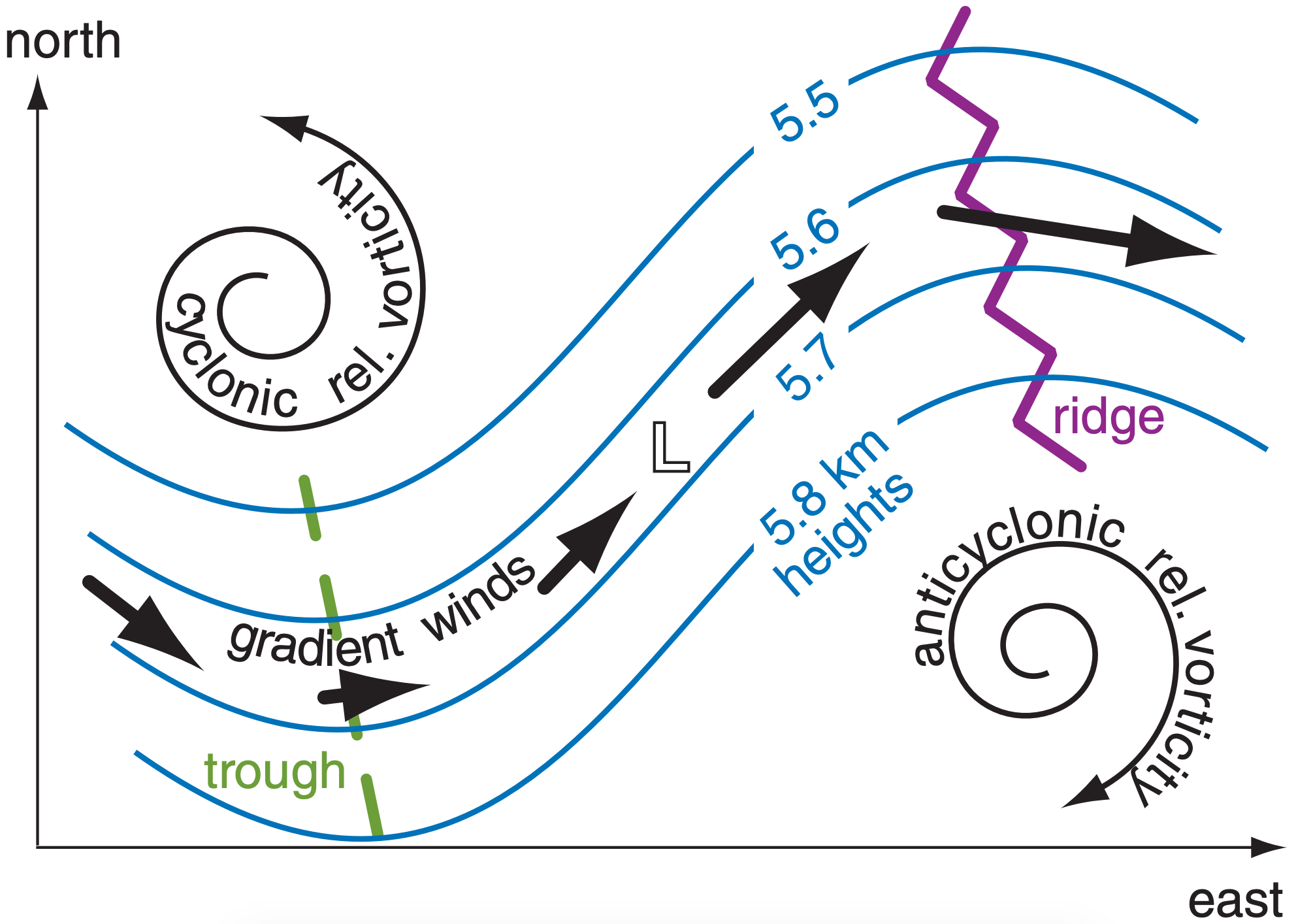
The beta term, however, contributes to spindown because air from lower latitudes (with smaller Coriolis parameter) is blowing toward the location of the surface cyclone. This effect is small when the wave amplitude is small. The sum of all three terms in the quasi-geostrophic vorticity equation is often positive, providing a net spin-up and intensification of the cyclone.
In real cyclones, contours are often more closely spaced in troughs, causing relative maxima in jet stream winds called jet streaks. Vertical motions associated with horizontal divergence in jet streaks are discussed later in this chapter. These motions violate the assumption that air mass is conserved along an “isobaric channel”. Rossby also pointed out in 1940 that the gradient wind balance is not valid for varying motions. Thus, the “toy” model of Fig. 13.27 has weaknesses that limit its applicability.
A Laplacian operator \(\nabla^{2}\) can be defined as
\(\nabla^{2} A=\dfrac{\partial^{2} A}{\partial x^{2}}+\dfrac{\partial^{2} A}{\partial y^{2}}+\dfrac{\partial^{2} A}{\partial z^{2}}\)
where A represents any variable. Sometimes we are concerned only with the horizontal (H) portion:
\(\nabla_{H}^{2}(A)=\dfrac{\partial^{2} A}{\partial x^{2}}+\dfrac{\partial^{2} A}{\partial y^{2}}\)
What does it mean? If ∂A/∂x represents the slope of a line when A is plotted vs. x on a graph, then ∂2A/∂x2 = ∂[ ∂A/∂x ]/∂x is the change of slope; namely, the curvature.
How is it used? Recall from the Atm. Forces & Winds chapter that the geostrophic wind is defined as
\(U_{g}=-\dfrac{1}{f_{c}} \dfrac{\partial \Phi}{\partial y} \quad\quad \quad V_{g}=\dfrac{1}{f_{c}} \dfrac{\partial \Phi}{\partial x}\)
or
\(\ \begin{align} \zeta_{g}=\dfrac{1}{f_{c}} \nabla_{H}^{2}(\Phi)\tag{13.11b}\end{align}\)
This illustrates the value of the Laplacian — as a way to more concisely describe the physics.
For example, a low-pressure center corresponds to a low-height center on an isobaric sfc. That isobaric surface is concave up, which corresponds to positive curvature. Namely, the Laplacian of |g|·z is positive, hence, ζg is positive. Thus, a low has positive vorticity