14.3: A Look at Some Real Data on Fractional Transport Rates, From the Flume and From the Field
- Page ID
- 4241
\( \newcommand{\vecs}[1]{\overset { \scriptstyle \rightharpoonup} {\mathbf{#1}} } \)
\( \newcommand{\vecd}[1]{\overset{-\!-\!\rightharpoonup}{\vphantom{a}\smash {#1}}} \)
\( \newcommand{\id}{\mathrm{id}}\) \( \newcommand{\Span}{\mathrm{span}}\)
( \newcommand{\kernel}{\mathrm{null}\,}\) \( \newcommand{\range}{\mathrm{range}\,}\)
\( \newcommand{\RealPart}{\mathrm{Re}}\) \( \newcommand{\ImaginaryPart}{\mathrm{Im}}\)
\( \newcommand{\Argument}{\mathrm{Arg}}\) \( \newcommand{\norm}[1]{\| #1 \|}\)
\( \newcommand{\inner}[2]{\langle #1, #2 \rangle}\)
\( \newcommand{\Span}{\mathrm{span}}\)
\( \newcommand{\id}{\mathrm{id}}\)
\( \newcommand{\Span}{\mathrm{span}}\)
\( \newcommand{\kernel}{\mathrm{null}\,}\)
\( \newcommand{\range}{\mathrm{range}\,}\)
\( \newcommand{\RealPart}{\mathrm{Re}}\)
\( \newcommand{\ImaginaryPart}{\mathrm{Im}}\)
\( \newcommand{\Argument}{\mathrm{Arg}}\)
\( \newcommand{\norm}[1]{\| #1 \|}\)
\( \newcommand{\inner}[2]{\langle #1, #2 \rangle}\)
\( \newcommand{\Span}{\mathrm{span}}\) \( \newcommand{\AA}{\unicode[.8,0]{x212B}}\)
\( \newcommand{\vectorA}[1]{\vec{#1}} % arrow\)
\( \newcommand{\vectorAt}[1]{\vec{\text{#1}}} % arrow\)
\( \newcommand{\vectorB}[1]{\overset { \scriptstyle \rightharpoonup} {\mathbf{#1}} } \)
\( \newcommand{\vectorC}[1]{\textbf{#1}} \)
\( \newcommand{\vectorD}[1]{\overrightarrow{#1}} \)
\( \newcommand{\vectorDt}[1]{\overrightarrow{\text{#1}}} \)
\( \newcommand{\vectE}[1]{\overset{-\!-\!\rightharpoonup}{\vphantom{a}\smash{\mathbf {#1}}}} \)
\( \newcommand{\vecs}[1]{\overset { \scriptstyle \rightharpoonup} {\mathbf{#1}} } \)
\( \newcommand{\vecd}[1]{\overset{-\!-\!\rightharpoonup}{\vphantom{a}\smash {#1}}} \)
\(\newcommand{\avec}{\mathbf a}\) \(\newcommand{\bvec}{\mathbf b}\) \(\newcommand{\cvec}{\mathbf c}\) \(\newcommand{\dvec}{\mathbf d}\) \(\newcommand{\dtil}{\widetilde{\mathbf d}}\) \(\newcommand{\evec}{\mathbf e}\) \(\newcommand{\fvec}{\mathbf f}\) \(\newcommand{\nvec}{\mathbf n}\) \(\newcommand{\pvec}{\mathbf p}\) \(\newcommand{\qvec}{\mathbf q}\) \(\newcommand{\svec}{\mathbf s}\) \(\newcommand{\tvec}{\mathbf t}\) \(\newcommand{\uvec}{\mathbf u}\) \(\newcommand{\vvec}{\mathbf v}\) \(\newcommand{\wvec}{\mathbf w}\) \(\newcommand{\xvec}{\mathbf x}\) \(\newcommand{\yvec}{\mathbf y}\) \(\newcommand{\zvec}{\mathbf z}\) \(\newcommand{\rvec}{\mathbf r}\) \(\newcommand{\mvec}{\mathbf m}\) \(\newcommand{\zerovec}{\mathbf 0}\) \(\newcommand{\onevec}{\mathbf 1}\) \(\newcommand{\real}{\mathbb R}\) \(\newcommand{\twovec}[2]{\left[\begin{array}{r}#1 \\ #2 \end{array}\right]}\) \(\newcommand{\ctwovec}[2]{\left[\begin{array}{c}#1 \\ #2 \end{array}\right]}\) \(\newcommand{\threevec}[3]{\left[\begin{array}{r}#1 \\ #2 \\ #3 \end{array}\right]}\) \(\newcommand{\cthreevec}[3]{\left[\begin{array}{c}#1 \\ #2 \\ #3 \end{array}\right]}\) \(\newcommand{\fourvec}[4]{\left[\begin{array}{r}#1 \\ #2 \\ #3 \\ #4 \end{array}\right]}\) \(\newcommand{\cfourvec}[4]{\left[\begin{array}{c}#1 \\ #2 \\ #3 \\ #4 \end{array}\right]}\) \(\newcommand{\fivevec}[5]{\left[\begin{array}{r}#1 \\ #2 \\ #3 \\ #4 \\ #5 \\ \end{array}\right]}\) \(\newcommand{\cfivevec}[5]{\left[\begin{array}{c}#1 \\ #2 \\ #3 \\ #4 \\ #5 \\ \end{array}\right]}\) \(\newcommand{\mattwo}[4]{\left[\begin{array}{rr}#1 \amp #2 \\ #3 \amp #4 \\ \end{array}\right]}\) \(\newcommand{\laspan}[1]{\text{Span}\{#1\}}\) \(\newcommand{\bcal}{\cal B}\) \(\newcommand{\ccal}{\cal C}\) \(\newcommand{\scal}{\cal S}\) \(\newcommand{\wcal}{\cal W}\) \(\newcommand{\ecal}{\cal E}\) \(\newcommand{\coords}[2]{\left\{#1\right\}_{#2}}\) \(\newcommand{\gray}[1]{\color{gray}{#1}}\) \(\newcommand{\lgray}[1]{\color{lightgray}{#1}}\) \(\newcommand{\rank}{\operatorname{rank}}\) \(\newcommand{\row}{\text{Row}}\) \(\newcommand{\col}{\text{Col}}\) \(\renewcommand{\row}{\text{Row}}\) \(\newcommand{\nul}{\text{Nul}}\) \(\newcommand{\var}{\text{Var}}\) \(\newcommand{\corr}{\text{corr}}\) \(\newcommand{\len}[1]{\left|#1\right|}\) \(\newcommand{\bbar}{\overline{\bvec}}\) \(\newcommand{\bhat}{\widehat{\bvec}}\) \(\newcommand{\bperp}{\bvec^\perp}\) \(\newcommand{\xhat}{\widehat{\xvec}}\) \(\newcommand{\vhat}{\widehat{\vvec}}\) \(\newcommand{\uhat}{\widehat{\uvec}}\) \(\newcommand{\what}{\widehat{\wvec}}\) \(\newcommand{\Sighat}{\widehat{\Sigma}}\) \(\newcommand{\lt}{<}\) \(\newcommand{\gt}{>}\) \(\newcommand{\amp}{&}\) \(\definecolor{fillinmathshade}{gray}{0.9}\)There has been a long-standing controversy over the reality or importance of equal mobility since the concept was first proposed by Parker et al. (1982b). Some sets of measurements, in flumes and in streams, have shown a close approach to equal mobility, whereas other studies have shown strong deviations from equal mobility.
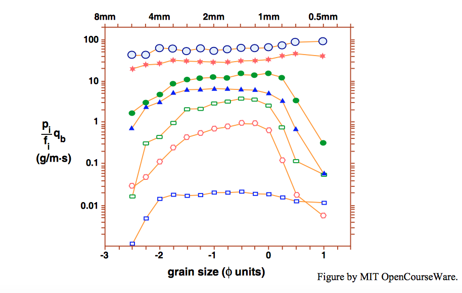
First we look at the results of the most revealing flume studies of fractional transport rates in unimodal sediment made up to now. Wilcock and Southard (1989) made a flume study of fractional transport rates in a sediment-recirculating flume. The sediment was of mixed size, with a mean size of \(1.83\) \(\mathrm{mm}\) and a unimodal distribution. In seven runs with increasing bed shear stress, the fractional bed-load transport rates of several size fractions, ranging in size from \(0.5\) \(\mathrm{mm}\) to \(6\) \(\mathrm{mm}\), were measured by use of a slot trap that extended across the width of the flume. Once weighed, the samples were returned to the system. Sampling was done at two times during a run: while the bed was still initially planar, and at a later time when the bed and the flow had reached equilibrium. In the runs at lower bed shear stress, the bed remained planar for the entire run, but at higher bed shear stresses, dunes developed on the bed.

You can see from Figure \(\PageIndex{1}\) (compare this figure with Figures 14.2.8 and 14.2.9) that for a wide range of size fractions in the middle part of the size distribution the fractional transport rates are nearly the same: in other words, there is a close approach to the condition of equal mobility for those size fractions. Except at the highest bed shear stresses, however, the curves depart from the conditions of equal mobility: the fractional transport rates of both the finest fractions and the coarsest fractions are more difficult to transport. You might have guessed that the coarsest fractions would be harder to transport, but it is somewhat surprising that the same is true for the finest fractions.

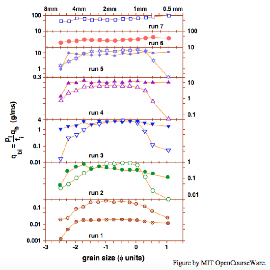
Figure \(\PageIndex{2}\), also from Wilcock and Southard (1988), repeats the data in Figure \(\PageIndex{1}\) but also shows the data for the initial conditions in the runs (except for the two at the highest bed shear stresses). The main difference in the data between the two conditions is that at the initial condition the finest fractions approach the condition of equal mobility more closely than they do at the equilibrium condition. The explanation seems to be lie in a combination of two effects:
- As time goes on, the finer particles find their way downward among the coarser particles to positions below the surface layer; and
- As a coarse pavements develops on the bed surface, the finer particles are hidden from the flow more effectively.
The most widely cited data set on fractional transport rates in natural streams is that of Milhous (1973) from Oak Creek, a gravel-bed stream in Oregon. The Oak Creek data were used by Parker et al. (1982b) in their classic work on the concept of equal mobility.
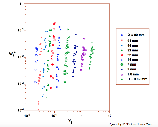
Figure \(\PageIndex{3}\), a graph of the Oak Creek data on fractional transport rate shows, unsurprisingly, that the fractional transport rates are a steeply increasing function of flow strength. The dimensionless version of the fractional transport rate, called the dimensionless bed-load parameter \(W_{i}^{*}\), is equal to \(\gamma^{\prime}q_{bvi}/f_{i}u_{*}^{3}\). (Note: the fractional transport rate, denoted here by \(q_{bvi}\), is by sediment volume, not sediment mass.) The reason for the separation of the curves for the various size fractions is that the dimensionless variable on the horizontal axis, \tau_{i}^{*} (= \tau_{\text{o}}/ \gamma^{\prime}D_i), contains the particle size \(D_{i}\) of the given fraction.

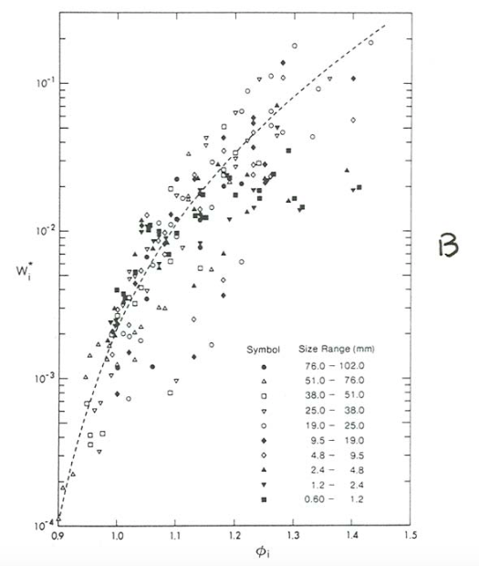
Each curve in Figure \(\PageIndex{3}\) was extrapolated downward to find the threshold shear stress, defined as the value for which \(W_{i}^{*}\) was at an arbitrarily chosen reference value of \(0.002\) (chosen to conform to what would match the commonly accepted condition of movement threshold; see the discussion on the reference-transport rate method of defining the movement threshold, in Chapter 9). Then, in a plot of \(W_{i}^{*}\) versus \(\tau^{*}_{r}/\tau^{*}_{ri}\), which Parker et al. denote by \(\phi_{i}\), all of the ten curves for fractional transport rate in Figure \(\PageIndex{3}\) collapse into a single curve—not perfectly, but to a fairly good approximation (Figure \(\PageIndex{4}\)).

(Here, the dimensionless variable \(\phi_{i} = tau^{*}_{r}/\tau^{*}_{ri}\) might need careful attention on your part: it is the reference value of the dimensionless bed shear stress at which the dimensionless total bed-load transport rate equals the reference total bed-load transport rate, divided by the reference value of the dimensionless bed shear stress of the \(i\)th size fraction at which the dimensionless bed-load transport rate of the \(i\)th fraction equals the reference bed-load transport rate of the \(i\)th fraction. (That long sentence requires careful reading.) Basically, it expresses the relative magnitude of the dimensionless bed shear stress at reference threshold condition for the bulk sediment, on the one hand, and the dimensionless bed shear stress at the reference condition for the \(i\)th fraction, on the other hand.)
What, then, is the significance of this “collapse” of the individual curves into a single curve? If you go back to the section on the thought experiment and look at Figure 14.2.7, for the condition of perfect equal mobility, you can see that Figure \(\PageIndex{4}\) is of the same nature, because the effect of having the particle size in the denominator of the dimensionless bed shear stress is circumvented by taking the ratio of the two dimensionless bed shear stresses. The conclusion to be drawn is that also in the case of this natural gravel-bed stream the condition of equal mobility is approached, although not met exactly. We must conclude, then, that the effects of hiding–sheltering and rollability combine, in some way, to make the transport of the various size fractions more nearly equal, when normalized by the proportions of the fractions in the mixture, although there still is a tendency for the coarser fractions to be less easily transported.


