14.2: Several Consequences of Size
- Page ID
- 4240
The Bed-Surface Size Distribution
If the flow is sufficiently strong, it moves some of the sediment that is resting on the bed surface. The question now arises: after the sediment transport reaches an equilibrium state, is the size distribution of the sediment on the bed surface the same as that of the sediment in the substrate? An unsophisticated observer might suppose, beforehand, that it would be the same. In general, however, it is not: it is coarser than the substrate. In part this develops because the flow selectively entrains the finer fractions in preference to the coarser fractions. In the sediment-transport literature, this has been termed selective entrainment. That should seem natural to you in light of what was said in Chapter 9, on movement threshold: it takes a stronger flow to move coarser sediment than it does to move finer sediment, so at first thought it might seem that in a mixed-size sediment the coarser fractions should be more difficult to move than the finer fractions.
There is another effect as well: the flow “develops” the bed surface as it works on it, in such a way that finer particles find their way down beneath coarser particles, leaving a bed-surface layer that is coarser than the underlying layers. Such a coarser surface layer, beneath a flow that is transporting the bed-material sediment in equilibrium, is called pavement (Parker and Klingeman, 1982; Parker et al., 1982a; Parker et al., 1982b). Pavement is similar to, but different from, armor, which is a coarse surface layer that develops as a flow winnows finer sediment to the point where no more sediment can be entrained by the flow. In other words, armor is a coarse bed-surface layer which, once it is formed, never moves, under ordinary circumstances (it could, of course, be disrupted by a rare, catastrophic event), whereas pavement is a coarse surface layer which, if not in equilibrium with the flow, is moved, at least in part, under ordinary circumstances. (By “ordinary circumstances” here I mean strong flow events that might occur during some number of time periods, small or large, in a typical year.)
Another way of thinking about the development of a coarse surface layer during bed-material transport is that, if the coarser fractions are more difficult to transport than the finer fractions, the concentration of those coarser fractions on the bed surface must increase, in order for the flow to transport the sediment it is given to transport. That is true to the extent that the sediment-transporting system is like a sediment-feed flume (See Chapter 8), for which the flow and the bed must become adjusted to transport the sediment that is fed, independently, into the flow at the upstream end of the flume.
Fractional Transport Rates
Suppose, now, that you measured the unit transport rate (that is, transport rate, in mass per unit time, per unit cross-stream width of the flow) of each size fraction in the mixture of transported sediment. These transport rates are called fractional transport rates, often denoted by \(q_{bi}\), where \(q\) represents the unit transport rate, the subscript \(i\) denotes the \(i\)th fraction in the mixture, and the subscript \(b\) stands for bed load or bed-material load. (In natural flow environments, of course, the size distribution is continuous, so you need to divide the size continuum, arbitrarily, into a large number of narrow fractions.)
You might measure the fractional transport rates in the following way—without great difficulty in a laboratory flume, but not without great difficulty, if not impossible, in a real stream or river! Build a slot trap of some kind across the flow at some station and extract all of the passing sediment during some interval of time. That might be called the “transport catch” (an unofficial term). If you divide the mass of the transport catch by the time interval and the width of the trap, you have the total unit transport rate, \(q_{b}\). Then sieve the transport catch into the various size fractions, to find the proportion \(p_{i}\) of each of the fractions in the catch, and multiply each of the \(p_{i}\) by the total transport rate \(q_{b}\) to find the fractional transport rates \(q_{bi}\). (That works well for the bed load, but much, if not most, of the suspended bed-material load is likely to pass over the trap. But the problem lies in practice, not in concept.)
Gradation Independence Versus Equal Mobility
For the relationships among the various fractional transport rates, you can think in terms of two end members. At one extreme, you might suppose that the transport of each size fraction is entirely independent of the presence of all of the other size fractions. Then the transport rate of each fraction could, in principle at least, be found by appeal to the same considerations that were described in the Chapter 13, on sediment transport rates. Such a situation might be called gradation independence. At the other extreme, you might suppose that, if you normalize the fractional transport rates by dividing them by the proportion \(f_{i}\) of the given fraction in the sediment bed all of the various fractions have the same normalized fractional transport rate; in other words, the ratio of the fractional transport rate of a given size fraction to the proportion of the given size fraction in the bed sediment is the same for all of the size fractions. Such a condition has been termed equal mobility.
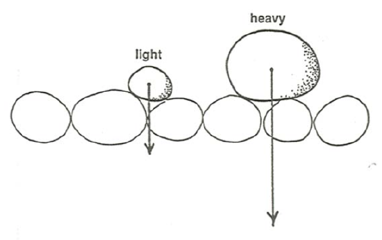
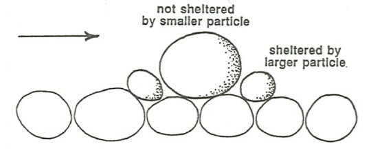
The condition of equal mobility might strike you as counterintuitive: should it not be more difficult for a flow to transport the coarser fractions than to transport the finer fractions? You might call this the particle-weight effect: larger particles are more difficult to move because they are heavier (Figure \(\PageIndex{1}\)). Two important countervailing effects tend to offset the particle-weight effect, though: (1) the hiding–sheltering effect, whereby larger particles are more exposed to the flow and thus have exerted on them a greater fluid force, but smaller particles tend to be sheltered from the forces of the flow by the larger particles (Figure \(\PageIndex{2}\)); and (2) the rollability effect, whereby larger particles can roll easily over a bed of smaller particles, but smaller particles cannot roll easily over a bed of larger particles (Figure \(\PageIndex{3}\)). The relative importance of the particle-weight effect, on the one hand, and the combination of the hiding– sheltering effect and the rollability effect, on the other hand, is an essential element in mixed-size sediment transport.
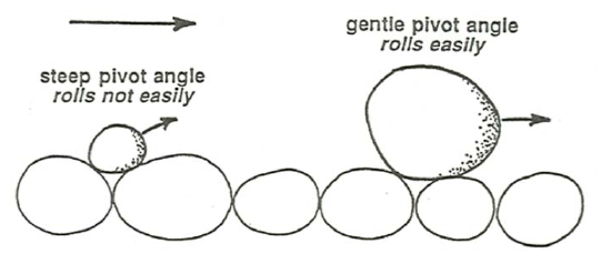
In the case of a sediment-feed flume (see Chapter 8), in which a bed of sediment is laid down and then a flow is passed over that bed while sediment that is identical to the bed sediment is fed at some rate at the upstream end of the flume, to be caught and discarded at the downstream end, the condition of equal mobility is forced upon the system, simply because the flow must transport all of the sediment it is given. Otherwise, the flow and sediment transport could never attain an equilibrium state. In order to transport the inherently more difficultly transportable fractions—the coarser fractions, presumably—the size distribution of the bed surface must become adjusted in such a way that the proportion of those difficultly transportable fractions on the bed surface are in greater proportion than they are in the underlying sediment bed. In a sediment- recirculating flume, by contrast, there is no such constraint: the flow is free to adjust its transport of the various size fractions in accordance with their inherent transportability. A fundamental question thus arises: to what extent does transport of mixed-size sediment in a sediment-recirculating flume approach the condition of equal mobility, even though that condition is not forced upon it? The reasons for the importance of that question is that natural rivers and streams, at least over short scales of space and time, seem to behave more like sediment- recirculating flumes than like sediment-feed flumes. The answer to that question will become apparent in a later section of this chapter.
A Thought Experiment to Demonstrate the Difference Between Gradation Dependence and Equal Mobility
Here is a hypothetical laboratory experiment to reveal more clearly for you the distinction between gradation independence and equal mobility. It would not be dauntingly difficult to do in an appropriately equipped sedimentation laboratory. Obtain or prepare three batches of sediment with nearly perfect sorting: classic “unisize” sediments. Their sizes might range from medium sand to fine gravel. Use each, in turn, for a series of flume runs to measure the unit sediment transport rate \(q_{b}\) (transport rate per unit width of flow), where the subscript \(b\) signifies bed-material load, over a wide range of boundary shear stresses \(\tau_{\text{o}}\), from only slightly above the threshold shear stress to a very large boundary shear stress, several times the threshold value. Plot graphs of \(q_{b}\) against \(\tau_{\text{o}}\) for each of the three sediments on a single graph (Figure \(\PageIndex{4}\)).
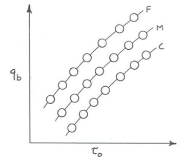
You know, beforehand, from the material in Chapter 12, what the graphs would look like, in an approximate way at least: for each sediment, the data points for the runs would fall on an approximately straight line in a \(\log-\log\) plot, with \(q_{b}\) increasing steeply with \(\tau_{\text{o}}\). The curve for the finest sediment would lie above that for the middle sediment, and the curve for the coarsest sediment would lie below that for the middle sediment—because the flow moves finer sediment more easily than coarser sediment.
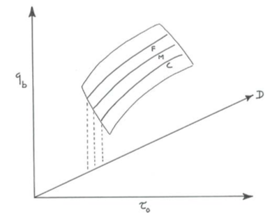
Another way of viewing the results graphically is to plot the results in a three-dimensional graph, by adding a third axis, the particle size (Figure \(\PageIndex{5}\)). Each of the three curves lies in its own plane, corresponding to position on the \(D\) axis. The earlier graph then is just a projection of the curves in those three separate planes onto the \(q_{b} –\tau_{\text{o}}\) axis plane.
Now mix the three unisize sediments together, to form a single starkly trimodal sediment mixture. Make a similar series of runs, with similar values of \(\tau_{\text{o}}\). For each value of \(\tau_{\text{o}}\), you need to compute the fractional transport rate of each of the three size fractions: \(q_{bi} = (p_{i}/f_{i})q_{b}\), where \(q_{b}\) is the total transport rate measured, \(p_{i}\) is the proportion of the transport rate (that is, the “transport catch”; see an earlier section) for the \(i\)th size fraction \((i = 1, 2, 3, \text{remember})\), and \(f_{i}\) is the proportion of the \(i\)th size fraction in the bulk sediment mixture you placed in the flume. Here we have normalized the \(q_{bi}\) by dividing by \(f_{i}\), to make clearest sense of the results. Again you can plot the results of \(q_{bi}\) in a three-dimensional graph, analogous to that in Figure \(\PageIndex{5}\), of \(q_{bi}\) vs. \(\tau_{\text{o}}\) and \(D_{i}\) (with \(D_{i}\) taking on three values—those of the modes of the trimodal particle-size distribution you created by mixing the three separate unisize batches).
Now the question is: what would the graph look like for the end- member cases of complete gradation independence, on the one hand, and perfect equal mobility, on the other hand?
(1) Gradation independence: In the case of gradation independence, if the \((p_{i}/f_{i})\) for the three fractions are what they would be in the absence of the other fractions—that is, each fraction behaves in transport without any interaction with the other size fractions—then the results would plot as three curves in the \(q_{b}– \tau_{\text{o}} –D_{i}\) graph, one curve in each of three \(D_{i} = \text{constant}\) planes just as with the graph for the separate batches, and the curves would be the same as before, after the change from \(q_{b}\) to \((p_{i}/f_{i})q_{b}\) is taken into account (Figure \(\PageIndex{6}\)).
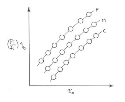
(2) Perfect equal mobility: In the case of perfect equal mobility, all of the normalized fractional transport rates are the same for a given value of \(\tau_{\text{o}}\): the transport dynamics of the various fractions are so closely interdependent that the transport rates of the various fractions are all the same, when adjusted for their proportions in the sediment mixture. In a graph of normalized fractional transport rate \((p_{i}/f_{i})q_{b}\) vs. \(\tau_{\text{o}}\) and \(D_{i}\) (Figure \(\PageIndex{7}\)), again there are three steeply rising curves, one for each value of \(D_{i}\), but now all three curves are the same, and when they are projected onto the \((p_{i}/f_{i})q_{b}– \tau_{\text{o}}\) plane, they fall on a single curve.
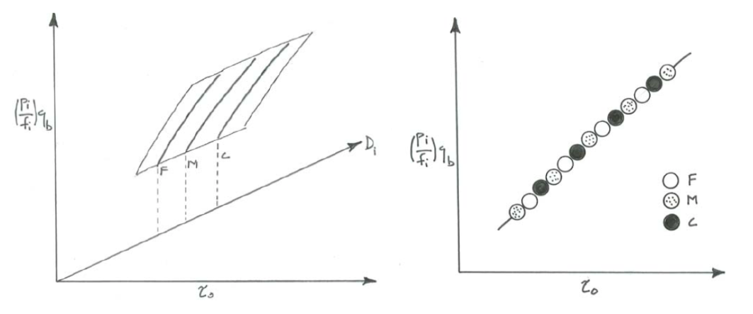
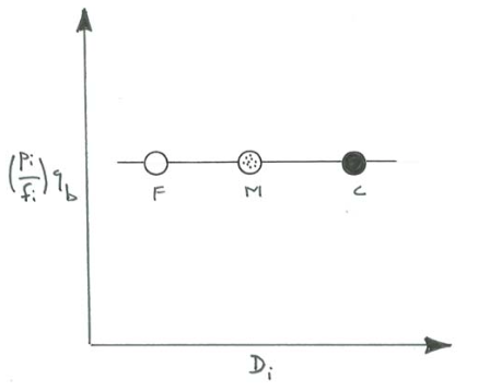
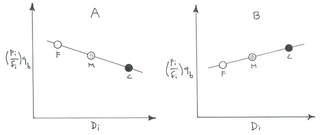
It is instructive to look also at how the three curves project onto the \((p_{i}/f_{i})q_{b}\) vs. \(D_{i}\) axis plane of the three-dimensional graph: with each value of \(\tau_{\text{o}}\) is associated a series of three points, and each of those sets of three points lies on a horizontal line, parallel to the \(D_{i}\) axis (Figure \(\PageIndex{8}\)). If the condition of equal mobility is not fulfilled, however, the curve would not be a horizontal line: if the fractional transport rates decrease with increasing sediment size, the curve would slope downward toward the coarser sizes (Figure \(\PageIndex{9}\)A) and if the fractional transport rates increase with increasing sediment size, the curve would slope upward toward the coarser sizes (Figure \(\PageIndex{9}\)B).
