14.4: Movement Threshold in Mixed-Sized Sediments
- Page ID
- 4242
\( \newcommand{\vecs}[1]{\overset { \scriptstyle \rightharpoonup} {\mathbf{#1}} } \)
\( \newcommand{\vecd}[1]{\overset{-\!-\!\rightharpoonup}{\vphantom{a}\smash {#1}}} \)
\( \newcommand{\dsum}{\displaystyle\sum\limits} \)
\( \newcommand{\dint}{\displaystyle\int\limits} \)
\( \newcommand{\dlim}{\displaystyle\lim\limits} \)
\( \newcommand{\id}{\mathrm{id}}\) \( \newcommand{\Span}{\mathrm{span}}\)
( \newcommand{\kernel}{\mathrm{null}\,}\) \( \newcommand{\range}{\mathrm{range}\,}\)
\( \newcommand{\RealPart}{\mathrm{Re}}\) \( \newcommand{\ImaginaryPart}{\mathrm{Im}}\)
\( \newcommand{\Argument}{\mathrm{Arg}}\) \( \newcommand{\norm}[1]{\| #1 \|}\)
\( \newcommand{\inner}[2]{\langle #1, #2 \rangle}\)
\( \newcommand{\Span}{\mathrm{span}}\)
\( \newcommand{\id}{\mathrm{id}}\)
\( \newcommand{\Span}{\mathrm{span}}\)
\( \newcommand{\kernel}{\mathrm{null}\,}\)
\( \newcommand{\range}{\mathrm{range}\,}\)
\( \newcommand{\RealPart}{\mathrm{Re}}\)
\( \newcommand{\ImaginaryPart}{\mathrm{Im}}\)
\( \newcommand{\Argument}{\mathrm{Arg}}\)
\( \newcommand{\norm}[1]{\| #1 \|}\)
\( \newcommand{\inner}[2]{\langle #1, #2 \rangle}\)
\( \newcommand{\Span}{\mathrm{span}}\) \( \newcommand{\AA}{\unicode[.8,0]{x212B}}\)
\( \newcommand{\vectorA}[1]{\vec{#1}} % arrow\)
\( \newcommand{\vectorAt}[1]{\vec{\text{#1}}} % arrow\)
\( \newcommand{\vectorB}[1]{\overset { \scriptstyle \rightharpoonup} {\mathbf{#1}} } \)
\( \newcommand{\vectorC}[1]{\textbf{#1}} \)
\( \newcommand{\vectorD}[1]{\overrightarrow{#1}} \)
\( \newcommand{\vectorDt}[1]{\overrightarrow{\text{#1}}} \)
\( \newcommand{\vectE}[1]{\overset{-\!-\!\rightharpoonup}{\vphantom{a}\smash{\mathbf {#1}}}} \)
\( \newcommand{\vecs}[1]{\overset { \scriptstyle \rightharpoonup} {\mathbf{#1}} } \)
\(\newcommand{\longvect}{\overrightarrow}\)
\( \newcommand{\vecd}[1]{\overset{-\!-\!\rightharpoonup}{\vphantom{a}\smash {#1}}} \)
\(\newcommand{\avec}{\mathbf a}\) \(\newcommand{\bvec}{\mathbf b}\) \(\newcommand{\cvec}{\mathbf c}\) \(\newcommand{\dvec}{\mathbf d}\) \(\newcommand{\dtil}{\widetilde{\mathbf d}}\) \(\newcommand{\evec}{\mathbf e}\) \(\newcommand{\fvec}{\mathbf f}\) \(\newcommand{\nvec}{\mathbf n}\) \(\newcommand{\pvec}{\mathbf p}\) \(\newcommand{\qvec}{\mathbf q}\) \(\newcommand{\svec}{\mathbf s}\) \(\newcommand{\tvec}{\mathbf t}\) \(\newcommand{\uvec}{\mathbf u}\) \(\newcommand{\vvec}{\mathbf v}\) \(\newcommand{\wvec}{\mathbf w}\) \(\newcommand{\xvec}{\mathbf x}\) \(\newcommand{\yvec}{\mathbf y}\) \(\newcommand{\zvec}{\mathbf z}\) \(\newcommand{\rvec}{\mathbf r}\) \(\newcommand{\mvec}{\mathbf m}\) \(\newcommand{\zerovec}{\mathbf 0}\) \(\newcommand{\onevec}{\mathbf 1}\) \(\newcommand{\real}{\mathbb R}\) \(\newcommand{\twovec}[2]{\left[\begin{array}{r}#1 \\ #2 \end{array}\right]}\) \(\newcommand{\ctwovec}[2]{\left[\begin{array}{c}#1 \\ #2 \end{array}\right]}\) \(\newcommand{\threevec}[3]{\left[\begin{array}{r}#1 \\ #2 \\ #3 \end{array}\right]}\) \(\newcommand{\cthreevec}[3]{\left[\begin{array}{c}#1 \\ #2 \\ #3 \end{array}\right]}\) \(\newcommand{\fourvec}[4]{\left[\begin{array}{r}#1 \\ #2 \\ #3 \\ #4 \end{array}\right]}\) \(\newcommand{\cfourvec}[4]{\left[\begin{array}{c}#1 \\ #2 \\ #3 \\ #4 \end{array}\right]}\) \(\newcommand{\fivevec}[5]{\left[\begin{array}{r}#1 \\ #2 \\ #3 \\ #4 \\ #5 \\ \end{array}\right]}\) \(\newcommand{\cfivevec}[5]{\left[\begin{array}{c}#1 \\ #2 \\ #3 \\ #4 \\ #5 \\ \end{array}\right]}\) \(\newcommand{\mattwo}[4]{\left[\begin{array}{rr}#1 \amp #2 \\ #3 \amp #4 \\ \end{array}\right]}\) \(\newcommand{\laspan}[1]{\text{Span}\{#1\}}\) \(\newcommand{\bcal}{\cal B}\) \(\newcommand{\ccal}{\cal C}\) \(\newcommand{\scal}{\cal S}\) \(\newcommand{\wcal}{\cal W}\) \(\newcommand{\ecal}{\cal E}\) \(\newcommand{\coords}[2]{\left\{#1\right\}_{#2}}\) \(\newcommand{\gray}[1]{\color{gray}{#1}}\) \(\newcommand{\lgray}[1]{\color{lightgray}{#1}}\) \(\newcommand{\rank}{\operatorname{rank}}\) \(\newcommand{\row}{\text{Row}}\) \(\newcommand{\col}{\text{Col}}\) \(\renewcommand{\row}{\text{Row}}\) \(\newcommand{\nul}{\text{Nul}}\) \(\newcommand{\var}{\text{Var}}\) \(\newcommand{\corr}{\text{corr}}\) \(\newcommand{\len}[1]{\left|#1\right|}\) \(\newcommand{\bbar}{\overline{\bvec}}\) \(\newcommand{\bhat}{\widehat{\bvec}}\) \(\newcommand{\bperp}{\bvec^\perp}\) \(\newcommand{\xhat}{\widehat{\xvec}}\) \(\newcommand{\vhat}{\widehat{\vvec}}\) \(\newcommand{\uhat}{\widehat{\uvec}}\) \(\newcommand{\what}{\widehat{\wvec}}\) \(\newcommand{\Sighat}{\widehat{\Sigma}}\) \(\newcommand{\lt}{<}\) \(\newcommand{\gt}{>}\) \(\newcommand{\amp}{&}\) \(\definecolor{fillinmathshade}{gray}{0.9}\)Introduction
It might seem like “putting the cart before the horse” to deal with movement thresholds after having already considered transport rates, but there is a certain logic to it, inasmuch as the most common way of identifying threshold conditions for mixed-size sediments is to measure transport rates for several values of boundary shear stress and then extrapolate downward to some chosen very low transport rate, called a reference transport rate, that corresponds approximately to what seems, by visual observations, to correspond to the boundary shear stress at which movement begins. The discussion in Chapter 9 on how to define the threshold condition in the first place is relevant here.
It is abundantly clear, from studies both in flumes and in natural flows, that the threshold shear stress for mixed-size sediments is different from that for unisize sediments. You should not expect to find that the threshold for movement of a certain size fraction in a mixed-size sediment is predictable by reference to the same sediment size in a relationship like the Shields diagram (Chapter 9), which is assumed to hold for unisize or very well-sorted sediment.
As with fractional transport rates, it is the outcome of the competition between the particle-weight effect, on the one hand, and the combination of the hiding–sheltering effect and the rollability effect, on the other hand, that is the key to movement threshold in mixed-size sediments. You should expect that to a first approximation the movement thresholds of the size fractions in a mixed-size sediment should be more nearly the same than would be predicted by, say, the Shields diagram for very well-sorted or unisize sediment. The question, again, as with fractional transport rates, is where the true situation lies between the end- member extremes of gradation independence (the threshold for each fraction is the same as for the same sizes of unisize sediment) and equal mobility (all of the size fractions of a mixed-size sediment begin to move at the same value of boundary shear stress).
Setting The Stage
Here is a useful framework for thinking about thresholds in mixed-size sediments, in light of what was just said about gradation independence and equal mobility:
Gradation independence: The threshold for each fraction is that same as if it were a unisize sediment, so \(\tau^{*}_{ci}\) \((\tau_{\text{o}c}/\gamma^{\prime}D_{i}\), the threshold value of the Shields parameter) is the same for all size fractions:
\[\tau^{*}_{ci} = \tau^{*}_{cj} \text{ for all } i, j \label{14.1} \]
We can massage this by setting, arbitrarily, \(\tau^{*}_{ci}\) equal to \(\tau^{*}_{c50}\), the threshold value for the \(50\)th percentile of the sediment mixture. That is,
\[ \tau_{ci}/\gamma^{\prime} D_{i} = \tau_{c50}/\gamma^{\prime} D_{50} \label{14.2} \]
Dividing both sides by \(\gamma^{\prime}\) and doing a bit of algebra then shows that
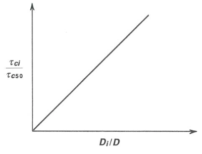
\[ \tau_{ci}/\tau_{c50} = D_{i}/D_{50} \label{14.3} \]
which expresses the condition of gradation independence. This would look like the graph in Figure \(\PageIndex{1}\). We can carry this a bit further by use of the definition of \(\tau^{*}: \tau_{ci} = \gamma^{\prime} D_{i}\tau^{*}_{ci}\) and \(\tau_{c50}= \gamma^{\prime} D_{50}\tau^{*}_{50}\), so the condition \(\tau_{ci}/\tau_{c50} = D_{i}/D_{50}\) can be written
\[\tau^{*}_{ci}/\tau^{*}_{c50} = 1 \label{14.4} \]
Equal mobility: each size fraction has the same movement threshold as all the others, and the particles of all of the size fractions start to move at the same value of \(\tau_{\text{o}}\):
\[\tau_{ci} = \tau_{cj} \text{ for all } i, j \label{14.5} \]
Again we can massage this by setting \(\tau_{ci}\) equal to \(\tau_{c50}\), for convenience, and then, with some algebra,
\[\tau_{ci}/\tau_{c50} = 1 \label{14.6} \]
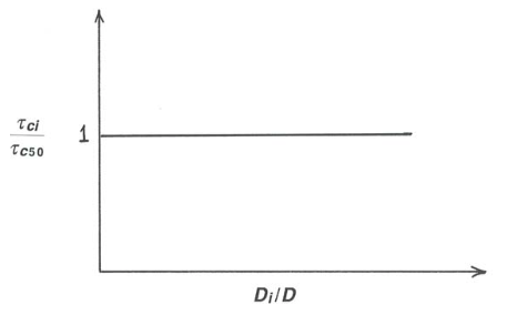
This would look like the graph in Figure \(\PageIndex{2}\). Again by use of the definition of \(\tau^{*}_{ci}\) and \(\tau^{*}_{c50}\), the condition \(\tau_{ci} = \tau_{c50}\) can be written
\[\tau^{*}_{ci}/\tau^{*}_{c50} = (D_{i}/D_{50}) -1 \label{14.7} \]
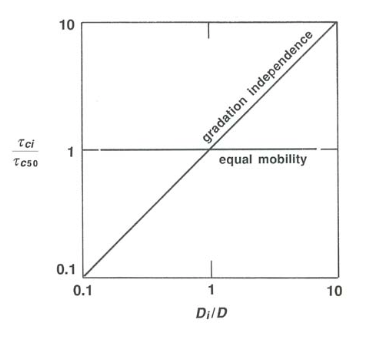
Finally, combining the results for both end-member cases, the contrast between gradation independence and equal mobility in graphic form is shown in Figures \(\PageIndex{3}\) and \(\PageIndex{4}\).
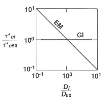
Some Real Data on Thresholds in Mixed-Sized Sediments
Wilcock and Southard (1988), using the same experimental arrangement described above for fractional transport rates, studied movement thresholds in five batches of mixed-size sediments, made up specifically to represent a range of median size and sorting. The three main batches were chosen to have mean size of about \(1.8\) \(\mathrm{mm}\) but with sorting ranging from very well sorted (phi standard deviation \(0.20\)) to moderately poorly sorted (phi standard deviation \(0.99\)). Also used were a well-sorted finer mixture, with mean size \(0.66\) \(\mathrm{mm}\), and a well-sorted coarser mixture, with mean size \(5.31\) \(\mathrm{mm}\). Movement threshold was determined by making several runs over a range of bed shear stress and extrapolating back to a reference transport rate chosen to correspond to a level of weak movement that would generally be agreed to represent threshold conditions.
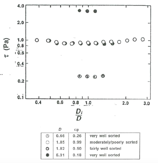
Figure \(\PageIndex{5}\) shows results for four of the sediment batches in a plot of \(\tau_{\text{o}}\) against \(D_{i}/D_{50}\), the ratio of the size of the given fraction to the mean size of the sediment batch. Owing to the differences in mean size, the curve for each sediment occupies a different range of \(\tau_{\text{o}}\), but what is interesting is that for each sediment the curves are nearly horizontal, indicating a close approach to equal mobility (see Equation \ref{14.6} and Figure \(\PageIndex{2}\) above).
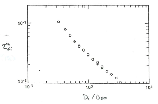
Figure \(\PageIndex{6}\) shows results for movement threshold in a plot of \(\tau^{*}_{ci}\), the dimensionless threshold bed shear stress for the \(i\)th fraction, against \(D_{i}/D\), the ratio of the size of the ith fraction to the mean size of the sediment batch. There are two noteworthy things about this graph:
- The downward trend of the curves shows that the results correspond to a condition close to equal mobility, which is that of a straight line with a slope of \(-1\) (compare with Equation \ref{14.7} and with the graph in Figure \(\PageIndex{2}\)B).
- The two curves are almost identical, showing that the sorting of the sediment has little effect on the thresholds of the individual size fractions, once \(D_{50}\) and relative size \(D_{i}/D_{50}\) are accounted for.
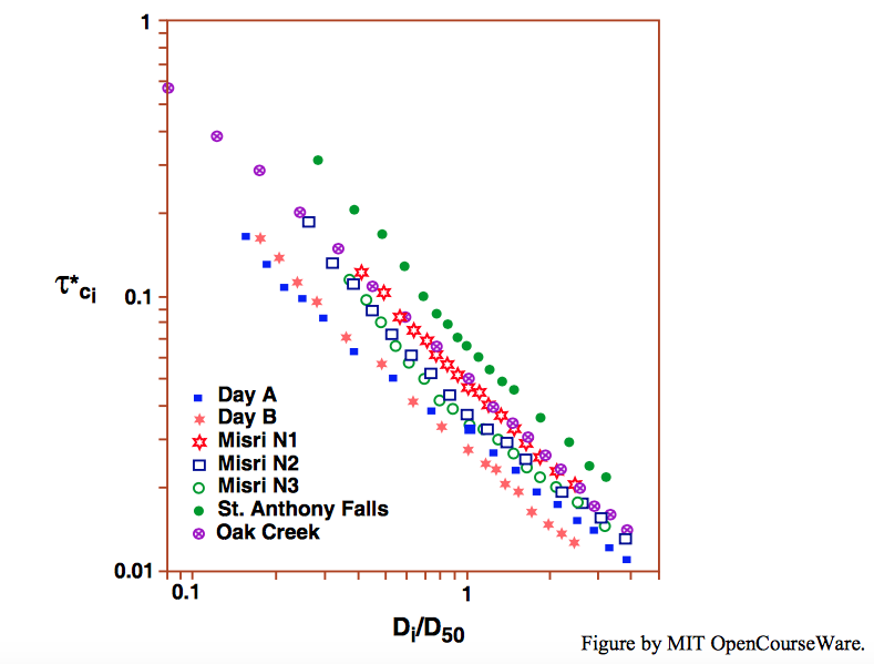
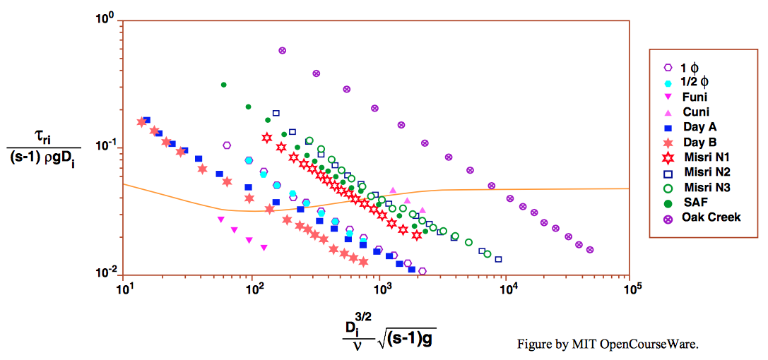
Figure \(\PageIndex{7}\) is a plot similar to that in Figure \(\PageIndex{6}\) for sediments from various laboratory and field studies. For these sediments as well, the condition of equal mobility, expressed as slope of \(-1\) in the plot, is approached but not met.
An equivalent, but revealing, way of presenting the data in Figure \(\PageIndex{7}\) is to plot (Figure \(\PageIndex{7}\)) the dimensionless threshold bed shear stress \(\tau^{*}_{ci}\) against the dimensionless variable \(D^{3} \gamma^{\prime} \rho/\mu^{2}\) (taken to the one-half power here), which is a nondimensionalization of the particle size in a way that does not involve the bed shear stress. The Shield curve for movement threshold is replotted in this graph as the solid curve. The downward slope of each of the curves defined by the data points shows clearly that the finer fractions of the sediment mixtures have threshold values that lie above the Shields curve, and the coarser fractions have threshold values that lie below the Shields curve.
