10.3: Transport Mode Versus Flow Intensity
- Page ID
- 4213
\( \newcommand{\vecs}[1]{\overset { \scriptstyle \rightharpoonup} {\mathbf{#1}} } \)
\( \newcommand{\vecd}[1]{\overset{-\!-\!\rightharpoonup}{\vphantom{a}\smash {#1}}} \)
\( \newcommand{\dsum}{\displaystyle\sum\limits} \)
\( \newcommand{\dint}{\displaystyle\int\limits} \)
\( \newcommand{\dlim}{\displaystyle\lim\limits} \)
\( \newcommand{\id}{\mathrm{id}}\) \( \newcommand{\Span}{\mathrm{span}}\)
( \newcommand{\kernel}{\mathrm{null}\,}\) \( \newcommand{\range}{\mathrm{range}\,}\)
\( \newcommand{\RealPart}{\mathrm{Re}}\) \( \newcommand{\ImaginaryPart}{\mathrm{Im}}\)
\( \newcommand{\Argument}{\mathrm{Arg}}\) \( \newcommand{\norm}[1]{\| #1 \|}\)
\( \newcommand{\inner}[2]{\langle #1, #2 \rangle}\)
\( \newcommand{\Span}{\mathrm{span}}\)
\( \newcommand{\id}{\mathrm{id}}\)
\( \newcommand{\Span}{\mathrm{span}}\)
\( \newcommand{\kernel}{\mathrm{null}\,}\)
\( \newcommand{\range}{\mathrm{range}\,}\)
\( \newcommand{\RealPart}{\mathrm{Re}}\)
\( \newcommand{\ImaginaryPart}{\mathrm{Im}}\)
\( \newcommand{\Argument}{\mathrm{Arg}}\)
\( \newcommand{\norm}[1]{\| #1 \|}\)
\( \newcommand{\inner}[2]{\langle #1, #2 \rangle}\)
\( \newcommand{\Span}{\mathrm{span}}\) \( \newcommand{\AA}{\unicode[.8,0]{x212B}}\)
\( \newcommand{\vectorA}[1]{\vec{#1}} % arrow\)
\( \newcommand{\vectorAt}[1]{\vec{\text{#1}}} % arrow\)
\( \newcommand{\vectorB}[1]{\overset { \scriptstyle \rightharpoonup} {\mathbf{#1}} } \)
\( \newcommand{\vectorC}[1]{\textbf{#1}} \)
\( \newcommand{\vectorD}[1]{\overrightarrow{#1}} \)
\( \newcommand{\vectorDt}[1]{\overrightarrow{\text{#1}}} \)
\( \newcommand{\vectE}[1]{\overset{-\!-\!\rightharpoonup}{\vphantom{a}\smash{\mathbf {#1}}}} \)
\( \newcommand{\vecs}[1]{\overset { \scriptstyle \rightharpoonup} {\mathbf{#1}} } \)
\(\newcommand{\longvect}{\overrightarrow}\)
\( \newcommand{\vecd}[1]{\overset{-\!-\!\rightharpoonup}{\vphantom{a}\smash {#1}}} \)
\(\newcommand{\avec}{\mathbf a}\) \(\newcommand{\bvec}{\mathbf b}\) \(\newcommand{\cvec}{\mathbf c}\) \(\newcommand{\dvec}{\mathbf d}\) \(\newcommand{\dtil}{\widetilde{\mathbf d}}\) \(\newcommand{\evec}{\mathbf e}\) \(\newcommand{\fvec}{\mathbf f}\) \(\newcommand{\nvec}{\mathbf n}\) \(\newcommand{\pvec}{\mathbf p}\) \(\newcommand{\qvec}{\mathbf q}\) \(\newcommand{\svec}{\mathbf s}\) \(\newcommand{\tvec}{\mathbf t}\) \(\newcommand{\uvec}{\mathbf u}\) \(\newcommand{\vvec}{\mathbf v}\) \(\newcommand{\wvec}{\mathbf w}\) \(\newcommand{\xvec}{\mathbf x}\) \(\newcommand{\yvec}{\mathbf y}\) \(\newcommand{\zvec}{\mathbf z}\) \(\newcommand{\rvec}{\mathbf r}\) \(\newcommand{\mvec}{\mathbf m}\) \(\newcommand{\zerovec}{\mathbf 0}\) \(\newcommand{\onevec}{\mathbf 1}\) \(\newcommand{\real}{\mathbb R}\) \(\newcommand{\twovec}[2]{\left[\begin{array}{r}#1 \\ #2 \end{array}\right]}\) \(\newcommand{\ctwovec}[2]{\left[\begin{array}{c}#1 \\ #2 \end{array}\right]}\) \(\newcommand{\threevec}[3]{\left[\begin{array}{r}#1 \\ #2 \\ #3 \end{array}\right]}\) \(\newcommand{\cthreevec}[3]{\left[\begin{array}{c}#1 \\ #2 \\ #3 \end{array}\right]}\) \(\newcommand{\fourvec}[4]{\left[\begin{array}{r}#1 \\ #2 \\ #3 \\ #4 \end{array}\right]}\) \(\newcommand{\cfourvec}[4]{\left[\begin{array}{c}#1 \\ #2 \\ #3 \\ #4 \end{array}\right]}\) \(\newcommand{\fivevec}[5]{\left[\begin{array}{r}#1 \\ #2 \\ #3 \\ #4 \\ #5 \\ \end{array}\right]}\) \(\newcommand{\cfivevec}[5]{\left[\begin{array}{c}#1 \\ #2 \\ #3 \\ #4 \\ #5 \\ \end{array}\right]}\) \(\newcommand{\mattwo}[4]{\left[\begin{array}{rr}#1 \amp #2 \\ #3 \amp #4 \\ \end{array}\right]}\) \(\newcommand{\laspan}[1]{\text{Span}\{#1\}}\) \(\newcommand{\bcal}{\cal B}\) \(\newcommand{\ccal}{\cal C}\) \(\newcommand{\scal}{\cal S}\) \(\newcommand{\wcal}{\cal W}\) \(\newcommand{\ecal}{\cal E}\) \(\newcommand{\coords}[2]{\left\{#1\right\}_{#2}}\) \(\newcommand{\gray}[1]{\color{gray}{#1}}\) \(\newcommand{\lgray}[1]{\color{lightgray}{#1}}\) \(\newcommand{\rank}{\operatorname{rank}}\) \(\newcommand{\row}{\text{Row}}\) \(\newcommand{\col}{\text{Col}}\) \(\renewcommand{\row}{\text{Row}}\) \(\newcommand{\nul}{\text{Nul}}\) \(\newcommand{\var}{\text{Var}}\) \(\newcommand{\corr}{\text{corr}}\) \(\newcommand{\len}[1]{\left|#1\right|}\) \(\newcommand{\bbar}{\overline{\bvec}}\) \(\newcommand{\bhat}{\widehat{\bvec}}\) \(\newcommand{\bperp}{\bvec^\perp}\) \(\newcommand{\xhat}{\widehat{\xvec}}\) \(\newcommand{\vhat}{\widehat{\vvec}}\) \(\newcommand{\uhat}{\widehat{\uvec}}\) \(\newcommand{\what}{\widehat{\wvec}}\) \(\newcommand{\Sighat}{\widehat{\Sigma}}\) \(\newcommand{\lt}{<}\) \(\newcommand{\gt}{>}\) \(\newcommand{\amp}{&}\) \(\definecolor{fillinmathshade}{gray}{0.9}\)Before we go into more detail about how sediment particles move, as bed load or in suspension or in saltation, it is worth developing a rational framework for relating the various modes of movement to one another. As with so many aspects of sediment transport, it is valuable to think in terms of regimes: distinctive ranges of the phenomenon, characterized by modes of particle movement that differ from other ranges. In this case, such regimes have been called transport stages. To develop a good framework for visualizing and assessing the results of experiments on transport stages, start by making a list of the variables that are likely to be important in determining the transport stage. The flow strength is best defined by the bed shear stress, just as it is for the threshold of movement. In contrast to the problem of movement threshold, however, the flow depth, which reflects the possible effects of outer-layer flow phenomena like large-scale turbulence (see Chapter 4), might not be ignorable, but as a first approximation suppose that the flow is characterized only by \(\tau_{\text{o}}\). Both particle size \(D\) and particle density \(\rho_{s}\) need to be included. The submerged specific weight of the particles, \(\gamma^{\prime}\), must be included as well as the particle density \(\rho_{s}\), because of the effect of particle weight in settling, aside from the effect of particle inertia when the particles experience accelerations caused by fluid turbulence. The fluid properties \(\rho\) and \(\mu\) have to be included for the usual reasons. Then
\[\text{transport stage} =f\left(\tau_{\text{o}}, D, \rho, \mu, \rho_{s}, \gamma^{\prime}\right) \label{10.1} \]
and we should expect that everything about the transport stage, expressed in dimensionless form, should be expressible in terms of three dimensionless variables. Examples of such things are: the positions of boundaries or boundary zones between qualitatively different transport stages; lengths or heights of particle trajectories, nondimensionalized by dividing by the particle diameter \(D\); or particle velocities, nondimensionalized by dividing by the shear velocity \(u_{*}\).
One such set of dimensionless variables might be:
- \(\left(\tau_{\text{o}}\right)^{\text{o}}=\left(\rho / \gamma^{\prime} \mu^{2}\right)^{1 / 3} \tau_{\text{o}}\), a dimensionless form of \(\tau_{\text{o}}\)
- \(\mathrm{D}^{\text{o}}=\left(\rho \gamma^{\prime} / \mu^{2}\right)^{1 / 3} D\), a dimensionless form of the particle diameter \(D\)
- \(\rho_{s} / \rho\)
The advantage of this set is that the leading variables, \(\tau_{\text{o}}\) and \(D\), are segregated into different dimensionless variables. An alternative would be to replace the dimensionless boundary shear stress with the flow intensity, \(u_{*}/u_{*c}\). In either case, one could attempt to plot experimental or theoretical results in two-dimensional graphs for certain values of \(\rho_{s} /\rho\) (most importantly, quartz-density sediment in water-density fluid).
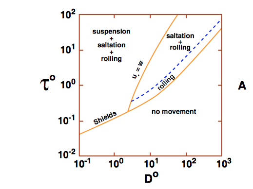
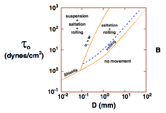
Figure \(\PageIndex{1}\), a very generalized version of a graph of boundary shear stress vs. particle size, makes a start at representing transport stages. In Figure \(\PageIndex{1}\), the axes are labeled in two ways: the dimensionless versions of \(\tau_{\text{o}}\) and \(D\) mentioned above, and also actual values of \(\tau_{\text{o}}\) and \(D\) at a water temperature of \(10^{\circ}\mathrm{C}\), to give a more concrete appreciation of conditions. We know at the outset that one boundary has to be present in the graph: the curve for threshold of particle motion. That is readily obtained by transforming the Shields curve (see Chapter 9) into these coordinates. Another boundary, which we consider next, is the curve for the onset of suspension in addition to bed-load movement.


The natural criterion for suspension is that the vertical turbulent velocities are at least as large as the settling velocities of the sediment particles; otherwise, particles could never be carried any higher above the bed than the entraining forces permit. The problem is that although for a given sediment size the settling velocity is fairly well defined (if effects of sorting and particle shape are ignored), the vertical turbulent velocities are distributed over a wide range of values. Should we use the very largest but very uncommon values, or smaller but more frequent values? What has commonly been done is to assume that the root-mean-square (\(\mathrm{rms}\)) value of the vertical turbulent velocities is a good measure to use. Measurements in turbulent boundary-layer flows past both smooth and rough boundaries have shown that there is a maximum close to the bed and that the maximum values reached are proportional to the shear velocity \(u_{*}\) (Blinco and Patheniades, 1971). The data of McQuivey and Richardson (1969) and Antonia and Luxton (1971) show that the maximum value of \((\mathrm{rms}\) \(v) / u_{*}\) is approximately equal to one and that the value does not depend strongly on the type of roughness. An approximate criterion for the onset of suspension is then
\[u_{*}=w \label{10.2} \]
For values of \(u_{*}\) less than \(w\), there should be no suspension, and for values of \(u_{*}\) greater than \(w\), some of the sediment should be traveling as suspended load. There is no reason to expect, however, that the coefficient of proportionality in Equation \ref{10.2} is exactly equal to one; the coefficient would presumably need to be adjusted somewhat in light of actual observations on the onset of suspension. Middleton (1976) has argued that the criterion \(u_{*} > w\) is also supported by a comparison of hydraulic measurements with the settling velocity of the largest particle sizes present in the suspended load of several rivers.
What remains is to convert the suspension criterion in Equation \ref{10.2} to a corresponding curve in Figure \(\PageIndex{1}\). To do this, first write Equation \ref{10.2} as
\[\left[\left(\tau_{\text{o}}\right)^{\text{o}}\right]^{1 / 2}=w^{\text{o}} \label{10.3} \]
by use of the definition of \(u_{*}\). Then use the definition of the dimensionless boundary shear stress \(\left(\tau_{\text{o}}\right)^{\text{o}}\) , given above, and a corresponding definition of dimensionless settling velocity, \(w^{\text{o}}=\left(\rho^{2} / \gamma^{\prime} \mu\right)^{1 / 3} w\) (see Chapter 2) to obtain an expression for \(\tau_{\text{o}}\) in terms of \(\left(\tau_{\text{o}}\right)^{\text{o}}\) and an expression for \(w\) in terms of \(w^{\text{o}}\):
\begin{equation}
\begin{array}{l}{\tau_{\text{o}}=\left(\frac{\gamma^{\prime2}\mu^{2}}{\rho}\right)^{1/3}\left(\tau_{\text{o}}\right)^{\text{o}}}\\ {w=\left(\frac{\gamma^{\prime} \mu}{\rho^{2}}\right) w^{\text{o}}}\end{array} \label{10.4}
\end{equation}
Now substitute the expressions for \(\tau_{\text{o}}\) and \(w\) in Equation \ref{10.4} into Equation \ref{10.3}:
\begin{equation}\left[\left(\frac{\gamma^{\prime2} \mu^{2}}{\rho}\right)\left(\tau_{0}\right)^{0}\right]^{1 / 3}=\rho^{1 / 2}\left[\left(\frac{\gamma^{\prime} \mu}{\rho^{2}}\right)^{1 / 3} w_{0}\right] \label{10.5} \end{equation}
and simplify to obtain
\begin{equation}\tau_{\text{o}}^{1 / 2}=\rho^{1 / 2} w \label{10.6} \end{equation}
The final step is to use the curve for \(w_{\text{o}}\) as a function of \(D_{\text{o}}\) (Figure 3.9.3 in Chapter 3) to obtain the relationship between \(\left(\tau_{\text{o}}\right)^{\text{o}}\) and \(D_{\text{o}}\) corresponding to the criterion for suspension:
\[\left[\left(\tau_{0}\right)^{0}\right]^{1 / 2}=f\left(D^{0}\right) \label{10.7} \]
Keep in mind that over most of its range, for settling-velocity Reynolds numbers greater than the Stokes range, the function in Equation \ref{10.7} has to be determined by observation.
We see that the curve that represents the suspension criterion slopes more steeply than the curve for incipient movement. This is just a manifestation of the fact that, qualitatively, the shear stress needed to make \(\mathrm{rms}\) \(v\) equal to the settling velocity with increasing particle size increases more rapidly than does the shear stress needed for incipient movement with increasing particle size. The consequence is that the two curves intersect at a certain small value of dimensionless particle size. (The suspension-inception curve does not extend downward below the movement-inception curve, because the flow there is not strong enough to move any sediment in the first place.) To the left of the intersection point, the fall velocity of the sediment particles is exceeded by the magnitude of the turbulent velocity fluctuations in the flow even at flow strengths just sufficient for sediment movement, so that sediment particles can be put into suspension as soon as they begin to be moved. Keep in mind, however, that at this and even finer sediment sizes, some of the sediment moves as bed load as well as suspended load. The existence of current ripples in sediments effectively at least as fine as medium silt is a good indication of this, inasmuch as ripples owe their existence to bed-load transport; see Chapter 12.
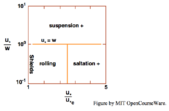
Finally, Figure \(\PageIndex{2}\), which shows transport stages in a graph of \(u_{*}/w\), the ratio of to shear velocity \(u_{*}\) to settling velocity \(w\) vs. flow intensity \(u_{*}/u_{*c}\) is an equivalent form of Figure \(\PageIndex{1}\); it is just a rubber-sheeted \(D^{\text{o}}-\tau^{\text{o}}\) diagram. It is neater and more synthetic than Figure \(\PageIndex{1}\), although perhaps less useful. Because \(w=f(D)\) and \(w \neq f\left(u_{*} / u_{* c}\right)\), there is a one-to-one correspondence between sediment diameter \(D\) and points on a vertical line in this graph. The movement-inception curve becomes the left-hand vertical axis \(\left(u_{*}=u_{* c}\right)\), and the suspension-inception criterion, \(u_{*}=w\), becomes a horizontal line. The area below the line for the suspension-inception criterion represents only bed-load transport, and the area above the line represents bed-load and suspended-load transport together.


