13.3: Predicting the Sediment Transport Rate

The Variables that Govern the Unit Sediment Transport Rate

It should seem natural to you to make a list of all of the important variables and physical effects that govern the sediment transport rate. Once we have such a list, we can frame our consideration of the sediment transport rate by expressing the sediment transport rate, in dimensionless form, in terms of a natural or convenient set of governing dimensionless variables. Even if for no other reason, such a functional relationship should guide your thinking about the various sediment-discharge formulas you might encounter in the literature on sediment transport.

Here is a list of the important physical effects on sediment transport rate, together with the variables associated with those physical effects; see Figure \(\PageIndex{1}\).

• Fluid forces on bed-surface particles: This is what moves the sediment. These fluid forces involve the bed shear stress \(\tau_{\text{o}}\), the fluid properties \(\rho\) and \(\mu\), and the particle size \(D\).
• The submerged weight of the particles is what resists the forces that tend to cause particle movement. It depends on the submerged specific weight of the particles, \(\gamma^{\prime}\) , and the particle size \(D\).
• The relative inertia of the sediment particles might have an effect on the sediment transport rate. It depends on the density of the sediment, \(\rho_{s}\), and the density of the fluid, \(\rho\).
• Turbulent diffusion of particles is important by virtue of its role in distribution sediment in suspension upward in the turbulent flow. It depends on a number of variables (Figure \(\PageIndex{1}\)).
• Fluid forces on particles in motion also depends upon a number of variables (Figure \(\PageIndex{1}\)).
• The presence of bed forms has an important effect on the sediment transport rate. As you saw in Chapter 11, that depends on a long list of variables (Figure \(\PageIndex{1}\)).

Figure \(\PageIndex{1}\): Important physical effects governing the unit sediment transport rate \(q_{s}\).

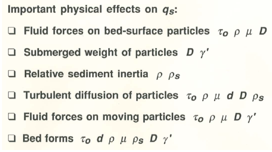
If we collect all of the variables in the above list, we see that each of the seven variables \(\tau_{\text{o}}\), \(d\), \(\rho\), \(\mu\), \(\rho_{s}\), \(D\), and \(\gamma^{\prime}\) appears somewhere in the list. Additionally, the effects of the joint size–shape–density (“SSD”) frequency distribution of the sediment are not taken into account by these seven variables. So we can express the dependence of \(q_{s}\) on these variables as

\[q_{s} = f(\tau_{\text{o}}, d, \rho, \mu, \rho_{s}, D, \gamma^{\prime}, \text{SSD distribution}) \label{12.1} \]

If we make the simplifying assumption that the SSD distribution is adequately represented by the mean or median size \(D\) and the standard deviation \(\sigma\), then \(q_{s}\) is a function of no fewer than eight governing variables:

\[q_{s} = f(\tau_{\text{o}}, d, \rho, \mu, \rho_{s}, D, \sigma, \gamma^{\prime}) \label{12.2} \]

Then, nondimensionalizing in a physically revealing way, an appropriate nondimensionalized sediment transport rate can be expressed as a function of five governing dimensionless variables:

\[ \frac{q_{s}}{\left(\rho \gamma^{\prime} D \right)^{1/2}} = f\left( \frac{\tau_{\text{o}}}{\gamma^{\prime}D}, \frac{\rho u_{*}D }{\mu}, \frac{d}{D}, \frac{\sigma}{D}.\frac{\rho_{s}}{\rho} \right) \label{12.3} \]

Here we have chosen to nondimensionalize the unit sediment transport rate by use of \(D\) rather than \(\tau_{\text{o}}\), although it is more common, in the literature on sediment transport, to do the latter. The most important governing independent dimensionless variable (which might be called the “leading variable”, is the first, the Shields parameter; see Chapter 9. The next two, the boundary Reynolds number and the relative roughness, express the turbulent structure of the flow. An alternative nondimensionalization might segregate the boundary shear stress and the median particle size into separate dimensionless variables.

Clearly, the list of governing dimensionless variables is unworkably long. It can be simplified in the following ways. If we restrict consideration to quartz-density sand in water, the density ratio becomes irrelevant, and if we restrict consideration to well-sorted sediments, the dimensionless sorting becomes unimportant. If we consider only flows for which the particle size is much smaller than the flow depth (that leaves out all white-water mountain streams), then we can safely omit the relative roughness from the list. That leaves two important variables, expressing the importance of the boundary shear stress and the median particle size. (Our intuition would have told us, in the first place, that the sediment transport rate should depend mainly on the force that moves the particles, and the size, and thus the weight, of the particles!) Most, if not all, of the various sediment-discharge formulas that have been proposed make use of one or both of the boundary shear stress and the particle size, in one or another form.

Sediment-Discharge Formulas

To an untutored observer, the most natural way of developing a sediment-discharge formula would be to start from the equations of motion (the Navier-Stokes equations) for turbulent sediment-transporting flow. There are two severe problems in that, however:

1. The turbulence closure problem (see Chapter 4) makes it impossible to work from first principles without making certain assumptions, and
2. The complexity of the physics of particle transport in turbulent shear flows means that the physics of the sediment transport cannot be supplied in a fundamental way.

What is commonly done, in the face of these difficulties, is first to attempt to adduce a rational dynamical basis for the sediment-transport process as a kind of framework, which results in one or more equations with certain adjustable parameters, and then use judiciously chosen data sets on measured sediment transport rates, from laboratory or field studies, to fit the equations to the data. (The ideal, of course, would be to have an equation with no adjustable parameters; a function with three or more adjustable parameters could be fitted to almost any data set!) The problem is that there is then no guarantee that the given sediment-discharge formula will work particularly well outside the range of data on which it was based.

The first modern attempt to develop a sediment discharge formula dates way back to DuBoys, in 1879. In the course of the twentieth century, a great many sediment-discharge formulas were proposed. Several of those have been widely used. If you go into the literature on sediment-transport rates, you will repeatedly encounter the names of certain workers, mainly hydraulic engineers, whose names are associated with sediment-discharge formulas: Einstein (Hans Albert, not the more famous father, Albert); Meyer–Peter and Müller; Bagnold; Engelund and Hansen.

These course notes are not the place to describe the various widely used sediment-discharge formulas. Vanoni (1975) gives brief descriptions of several such formulas. Here I will concentrate only upon comparisons among those formulas. Three useful comparison studies have appeared in the literature: Vanoni (1975), Gomez and Church (1989), and Nakato (1990).

Comparison of the Various Sediment-Discharge Formulas

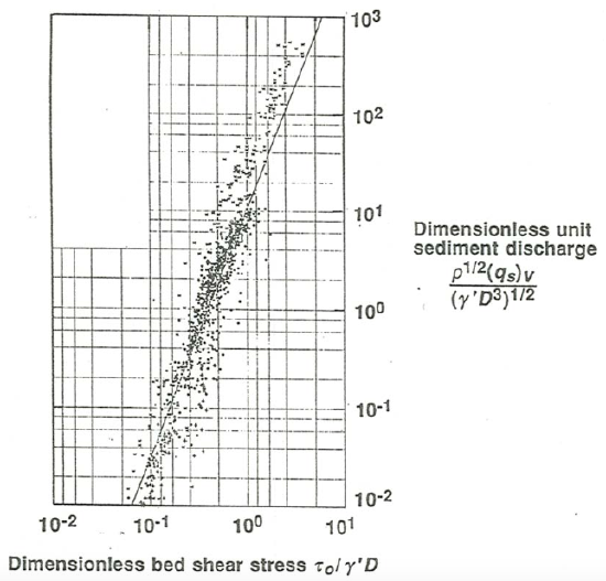
First, what do the data on sediment transport rate look like? Figure \(\PageIndex{2}\) is a plot of dimensionless unit sediment transport rate, nondimensionalized by use of sediment size \(D\), fluid density \(\rho\), and submerged specific weight of the sediment, \(\gamma^{\prime}\), against a dimensionless measure of the boundary shear stress, the Shields parameter \(\tau_{\text{o}}/ \gamma^{\prime} D\). The data are from both laboratory studies and measurements in rivers. In this undistorted log–log plot, you can see clearly the following:

• The sediment transport rate is a very steeply increasing function of the boundary shear stress. From the slope of the best-fit line in the graph, the unit sediment transport rate goes approximately as the cube of the boundary shear stress.
• Over five orders of magnitude of the unit sediment transport rate, the data fall along a fairly well-defined trend.
• Nonetheless there is considerable scatter in the data: if you pick one value of the dimensionless boundary shear stress, then, even if you ignore outlying points, there is an approximately order-of magnitude (factor of ten) spread in the data points.

Figure \(\PageIndex{2}\): Plot of dimensionless unit sediment transport rate (expressed as volume, not mass) against dimensionless boundary shear stress (in the form of the Shields parameter) for various sets of measurement data. (Modified from Vanoni, 1975.)

This large spread in values should not surprise you, when you consider that

1. The effects of particle size distribution and of the variable presence of bed forms is not taken into account, and
2. As you saw above, it is difficult to make accurate measurements of the sediment transport rate.

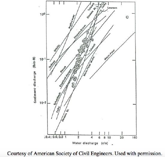
Figure \(\PageIndex{3}\) shows a comparison of the performance of several sediment-discharge formulas in accounting for a single high-quality set of measurements of unit sediment discharge. You can see that the various formulas vary greatly in how well they match the actual data. In fairness, however, I could point out that the conditions represented by this data set are far from the conditions for which some of the discharge formulas were derived. For example, the widely used Meyer–Peter formula was derived for coarse sediments, whereas the data set shown in the figure is for sand that falls just barely within the medium-sand range. The lesson here, I suppose, is that you cannot expect any sediment-discharge formula to work well outside the range for which it was conceived.

Figure \(\PageIndex{3}\): Sediment discharge against water discharge for the Niobrara River near Cody, Wyoming, U.S.A. obtained from observations (data points) and calculations on the basis of several sediment-discharge formulas (solid curves). (From Vanoni, 1975.)

Chapter 13 References Cited

Vanoni, V.A., ed., 1975, Sedimentation Engineering: American Society of Civil Engineers, Manuals and Reports on Engineering Practice, no. 54, 745 p.

Gomez, B., and Church, M., 1989, An assessment of bed load sediment transport: formulae for gravel bed rivers: Water Resources Research, v. 25, p. 1161- 1186.

Nakato, T., 1990, Tests of selected sediment-transport formulas: Journal of Hydraulic Engineering, v. 116, p. 362-379.