9.6.2: Equilibrium relations for tidal channels and flats
- Page ID
- 16408
\( \newcommand{\vecs}[1]{\overset { \scriptstyle \rightharpoonup} {\mathbf{#1}} } \)
\( \newcommand{\vecd}[1]{\overset{-\!-\!\rightharpoonup}{\vphantom{a}\smash {#1}}} \)
\( \newcommand{\id}{\mathrm{id}}\) \( \newcommand{\Span}{\mathrm{span}}\)
( \newcommand{\kernel}{\mathrm{null}\,}\) \( \newcommand{\range}{\mathrm{range}\,}\)
\( \newcommand{\RealPart}{\mathrm{Re}}\) \( \newcommand{\ImaginaryPart}{\mathrm{Im}}\)
\( \newcommand{\Argument}{\mathrm{Arg}}\) \( \newcommand{\norm}[1]{\| #1 \|}\)
\( \newcommand{\inner}[2]{\langle #1, #2 \rangle}\)
\( \newcommand{\Span}{\mathrm{span}}\)
\( \newcommand{\id}{\mathrm{id}}\)
\( \newcommand{\Span}{\mathrm{span}}\)
\( \newcommand{\kernel}{\mathrm{null}\,}\)
\( \newcommand{\range}{\mathrm{range}\,}\)
\( \newcommand{\RealPart}{\mathrm{Re}}\)
\( \newcommand{\ImaginaryPart}{\mathrm{Im}}\)
\( \newcommand{\Argument}{\mathrm{Arg}}\)
\( \newcommand{\norm}[1]{\| #1 \|}\)
\( \newcommand{\inner}[2]{\langle #1, #2 \rangle}\)
\( \newcommand{\Span}{\mathrm{span}}\) \( \newcommand{\AA}{\unicode[.8,0]{x212B}}\)
\( \newcommand{\vectorA}[1]{\vec{#1}} % arrow\)
\( \newcommand{\vectorAt}[1]{\vec{\text{#1}}} % arrow\)
\( \newcommand{\vectorB}[1]{\overset { \scriptstyle \rightharpoonup} {\mathbf{#1}} } \)
\( \newcommand{\vectorC}[1]{\textbf{#1}} \)
\( \newcommand{\vectorD}[1]{\overrightarrow{#1}} \)
\( \newcommand{\vectorDt}[1]{\overrightarrow{\text{#1}}} \)
\( \newcommand{\vectE}[1]{\overset{-\!-\!\rightharpoonup}{\vphantom{a}\smash{\mathbf {#1}}}} \)
\( \newcommand{\vecs}[1]{\overset { \scriptstyle \rightharpoonup} {\mathbf{#1}} } \)
\( \newcommand{\vecd}[1]{\overset{-\!-\!\rightharpoonup}{\vphantom{a}\smash {#1}}} \)
\(\newcommand{\avec}{\mathbf a}\) \(\newcommand{\bvec}{\mathbf b}\) \(\newcommand{\cvec}{\mathbf c}\) \(\newcommand{\dvec}{\mathbf d}\) \(\newcommand{\dtil}{\widetilde{\mathbf d}}\) \(\newcommand{\evec}{\mathbf e}\) \(\newcommand{\fvec}{\mathbf f}\) \(\newcommand{\nvec}{\mathbf n}\) \(\newcommand{\pvec}{\mathbf p}\) \(\newcommand{\qvec}{\mathbf q}\) \(\newcommand{\svec}{\mathbf s}\) \(\newcommand{\tvec}{\mathbf t}\) \(\newcommand{\uvec}{\mathbf u}\) \(\newcommand{\vvec}{\mathbf v}\) \(\newcommand{\wvec}{\mathbf w}\) \(\newcommand{\xvec}{\mathbf x}\) \(\newcommand{\yvec}{\mathbf y}\) \(\newcommand{\zvec}{\mathbf z}\) \(\newcommand{\rvec}{\mathbf r}\) \(\newcommand{\mvec}{\mathbf m}\) \(\newcommand{\zerovec}{\mathbf 0}\) \(\newcommand{\onevec}{\mathbf 1}\) \(\newcommand{\real}{\mathbb R}\) \(\newcommand{\twovec}[2]{\left[\begin{array}{r}#1 \\ #2 \end{array}\right]}\) \(\newcommand{\ctwovec}[2]{\left[\begin{array}{c}#1 \\ #2 \end{array}\right]}\) \(\newcommand{\threevec}[3]{\left[\begin{array}{r}#1 \\ #2 \\ #3 \end{array}\right]}\) \(\newcommand{\cthreevec}[3]{\left[\begin{array}{c}#1 \\ #2 \\ #3 \end{array}\right]}\) \(\newcommand{\fourvec}[4]{\left[\begin{array}{r}#1 \\ #2 \\ #3 \\ #4 \end{array}\right]}\) \(\newcommand{\cfourvec}[4]{\left[\begin{array}{c}#1 \\ #2 \\ #3 \\ #4 \end{array}\right]}\) \(\newcommand{\fivevec}[5]{\left[\begin{array}{r}#1 \\ #2 \\ #3 \\ #4 \\ #5 \\ \end{array}\right]}\) \(\newcommand{\cfivevec}[5]{\left[\begin{array}{c}#1 \\ #2 \\ #3 \\ #4 \\ #5 \\ \end{array}\right]}\) \(\newcommand{\mattwo}[4]{\left[\begin{array}{rr}#1 \amp #2 \\ #3 \amp #4 \\ \end{array}\right]}\) \(\newcommand{\laspan}[1]{\text{Span}\{#1\}}\) \(\newcommand{\bcal}{\cal B}\) \(\newcommand{\ccal}{\cal C}\) \(\newcommand{\scal}{\cal S}\) \(\newcommand{\wcal}{\cal W}\) \(\newcommand{\ecal}{\cal E}\) \(\newcommand{\coords}[2]{\left\{#1\right\}_{#2}}\) \(\newcommand{\gray}[1]{\color{gray}{#1}}\) \(\newcommand{\lgray}[1]{\color{lightgray}{#1}}\) \(\newcommand{\rank}{\operatorname{rank}}\) \(\newcommand{\row}{\text{Row}}\) \(\newcommand{\col}{\text{Col}}\) \(\renewcommand{\row}{\text{Row}}\) \(\newcommand{\nul}{\text{Nul}}\) \(\newcommand{\var}{\text{Var}}\) \(\newcommand{\corr}{\text{corr}}\) \(\newcommand{\len}[1]{\left|#1\right|}\) \(\newcommand{\bbar}{\overline{\bvec}}\) \(\newcommand{\bhat}{\widehat{\bvec}}\) \(\newcommand{\bperp}{\bvec^\perp}\) \(\newcommand{\xhat}{\widehat{\xvec}}\) \(\newcommand{\vhat}{\widehat{\vvec}}\) \(\newcommand{\uhat}{\widehat{\uvec}}\) \(\newcommand{\what}{\widehat{\wvec}}\) \(\newcommand{\Sighat}{\widehat{\Sigma}}\) \(\newcommand{\lt}{<}\) \(\newcommand{\gt}{>}\) \(\newcommand{\amp}{&}\) \(\definecolor{fillinmathshade}{gray}{0.9}\)The stability of the various morphological units of the inlet system can be described with empirical relations. These relationships relate geometric properties to hydraulic boundary conditions. In Sect. 9.5.2, we discussed the stability of the entrance of the inlet and described the cross-sectional area of the entrance as a function of the tidal prism. The sand volume stored in the ebb-tidal delta was discussed in Sect. 9.4.3 and could also be related to the tidal prism. In this section two other morphological units of an inlet and basin system are described: the tidal channels and tidal flats in the basin.
Equation 9.5.2.1 relates the equilibrium cross-sectional area in the throat, \(A_e\), to the tidal prism \(P\) (with \(q = 1\)). From data of a tidal channel in the Wadden Sea it appeared that also along a channel the flow area was related to the tidal volume passing the local cross-section. Later on it was found that for various tidal channels in the Wadden Sea and in the estuaries of the Delta in the southern Netherlands this relationship was valid. This relationship is given by:
\[A_{\text{MSL}} = C_A P_{AB}\label{eq9.6.2.1}\]
in which:
| \(A_{\text{MSL}}\) | the equilibrium flow area in a certain cross-section AB of the basin, measured below mean sea level | \(m^2\) |
| \(P_{AB}\) | the tidal prism landward of the cross-section AB under consideration | \(m^3\) |
| \(C_A\) | empirical coefficient | \(m^{-1}\) |
The tidal prism now is the tidal prism behind the cross-section under consideration (and not the total tidal prism for the entire basin). The flow area below MSL could be considered as the channel cross-sectional area \(A_c\). The flats are then defined as lying above MSL (but note that in other cases, they may be defined as lying above MLW).
In the case that the flood-tidal delta spans the entire basin area (as is the case for e.g. the Wadden Sea), an empirical relationship for the total basin channel volume is:
\[V_c = C_V P^{3/2}\label{eq9.6.2.2}\]
in which:
| \(V_c\) | the equilibrium total channel volume below below mean sea level | \(m^3\) |
| \(P\) | the tidal prism | \(m^3\) |
| \(C_V\) | empirical coefficient | \(m^{-3/2}\) |
For example, the empirical coefficient \(C_V\) is \(65 \times 10^{-6}\ m^{-3/2}\) for the Wadden Sea and \(73 \times 10^{-6}\ m^{-3/2}\) to \(80 \times 10^{-6}\ m^{-3/2}\) for the Eastern Scheldt and the Grevelingen (Eysink, 1991).
The power 3⁄2 in Eq. \(\ref{eq9.6.2.2}\) can be understood as follows. We have found that the cross- sectional area of the channels is proportional to the tidal prism (Eq. \(\ref{eq9.6.2.1}\)). Further, the length of the channels is proportional to the square root of the basin surface area (channels and flats), which in turn is proportional to the square root of the tidal prism. We then have:
\[\begin{array} {r} {A_c \propto P} \\ {L_c \propto \sqrt{A_b} \propto \sqrt{P}} \end{array} \Rightarrow V_c = A_c L_c \propto P \sqrt{A_b} \propto P^{3/2}\]
in which:
| \(A_c\) | the channel cross-section | \(m^2\) |
| \(P\) | the tidal prism | \(m^3\) |
| \(L_c\) | length of channels | \(m\) |
| \(V_c\) | volume of channels | \(m^3\) |
| \(A_b\) | the gross basin area (flats and channels) | \(m^2\) |

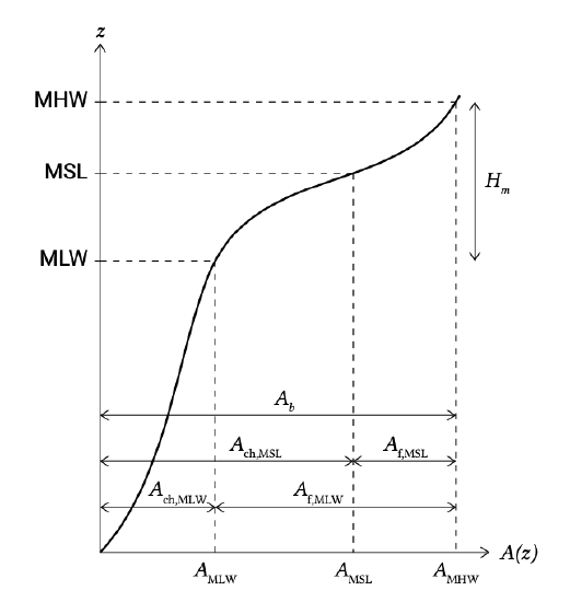
From the proportionalities of Eq. \(\ref{eq9.6.2.2}\), we can also deduce a relationship between the tidal flat area and the total basin area. The flats area is equal to the total basin area minus the channels area (Fig. 9.25):
\[A_f = A_b - A_{ch} = A_b - \dfrac{V_c}{D_c} \approx A_b - \alpha \dfrac{P \sqrt{A_b}}{D_c} \approx A_b - \beta \dfrac{H_m}{D_c} A_b^{3/2}\]
in which
| \(A_f\) | the flats' area i.e. the area above MSI. | \(m^2\) |
| \(A_{ch}\) | the horizontal area below MSL covered by all channels | \(m^2\) |
| \(\alpha, \beta\) | the horizontal area below MSL covered by all channels | \(m^{-1}\) |
| \(D_c\) | characteristic channel depth | \(m\) |
| \(H_m\) | mean tidal range | \(m\) |
Renger and Partenscky found for the German Bight:
\[A_f = A_b - 0.025 A_b^{3/2}\]

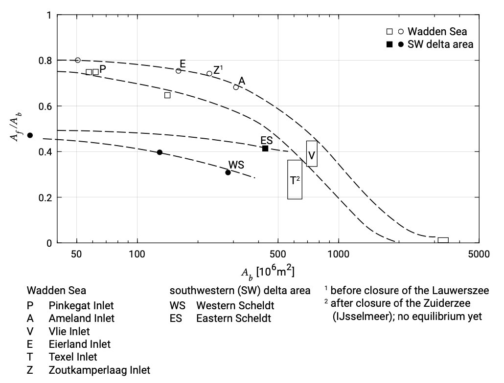
Figure 9.26 shows similar relationships for the estuaries in the south of the Netherlands and for the Wadden Sea basins. An explanation for the trend of the relation could be the increasing activity of local wind waves in larger basins (since waves act as an eroding agent on the flats).


