
9.5.2: Empirical equilibrium cross-sectional area
- Page ID
- 16406

\( \newcommand{\vecs}[1]{\overset { \scriptstyle \rightharpoonup} {\mathbf{#1}} } \)
\( \newcommand{\vecd}[1]{\overset{-\!-\!\rightharpoonup}{\vphantom{a}\smash {#1}}} \)
\( \newcommand{\id}{\mathrm{id}}\) \( \newcommand{\Span}{\mathrm{span}}\)
( \newcommand{\kernel}{\mathrm{null}\,}\) \( \newcommand{\range}{\mathrm{range}\,}\)
\( \newcommand{\RealPart}{\mathrm{Re}}\) \( \newcommand{\ImaginaryPart}{\mathrm{Im}}\)
\( \newcommand{\Argument}{\mathrm{Arg}}\) \( \newcommand{\norm}[1]{\| #1 \|}\)
\( \newcommand{\inner}[2]{\langle #1, #2 \rangle}\)
\( \newcommand{\Span}{\mathrm{span}}\)
\( \newcommand{\id}{\mathrm{id}}\)
\( \newcommand{\Span}{\mathrm{span}}\)
\( \newcommand{\kernel}{\mathrm{null}\,}\)
\( \newcommand{\range}{\mathrm{range}\,}\)
\( \newcommand{\RealPart}{\mathrm{Re}}\)
\( \newcommand{\ImaginaryPart}{\mathrm{Im}}\)
\( \newcommand{\Argument}{\mathrm{Arg}}\)
\( \newcommand{\norm}[1]{\| #1 \|}\)
\( \newcommand{\inner}[2]{\langle #1, #2 \rangle}\)
\( \newcommand{\Span}{\mathrm{span}}\) \( \newcommand{\AA}{\unicode[.8,0]{x212B}}\)
\( \newcommand{\vectorA}[1]{\vec{#1}} % arrow\)
\( \newcommand{\vectorAt}[1]{\vec{\text{#1}}} % arrow\)
\( \newcommand{\vectorB}[1]{\overset { \scriptstyle \rightharpoonup} {\mathbf{#1}} } \)
\( \newcommand{\vectorC}[1]{\textbf{#1}} \)
\( \newcommand{\vectorD}[1]{\overrightarrow{#1}} \)
\( \newcommand{\vectorDt}[1]{\overrightarrow{\text{#1}}} \)
\( \newcommand{\vectE}[1]{\overset{-\!-\!\rightharpoonup}{\vphantom{a}\smash{\mathbf {#1}}}} \)
\( \newcommand{\vecs}[1]{\overset { \scriptstyle \rightharpoonup} {\mathbf{#1}} } \)
\( \newcommand{\vecd}[1]{\overset{-\!-\!\rightharpoonup}{\vphantom{a}\smash {#1}}} \)
\(\newcommand{\avec}{\mathbf a}\) \(\newcommand{\bvec}{\mathbf b}\) \(\newcommand{\cvec}{\mathbf c}\) \(\newcommand{\dvec}{\mathbf d}\) \(\newcommand{\dtil}{\widetilde{\mathbf d}}\) \(\newcommand{\evec}{\mathbf e}\) \(\newcommand{\fvec}{\mathbf f}\) \(\newcommand{\nvec}{\mathbf n}\) \(\newcommand{\pvec}{\mathbf p}\) \(\newcommand{\qvec}{\mathbf q}\) \(\newcommand{\svec}{\mathbf s}\) \(\newcommand{\tvec}{\mathbf t}\) \(\newcommand{\uvec}{\mathbf u}\) \(\newcommand{\vvec}{\mathbf v}\) \(\newcommand{\wvec}{\mathbf w}\) \(\newcommand{\xvec}{\mathbf x}\) \(\newcommand{\yvec}{\mathbf y}\) \(\newcommand{\zvec}{\mathbf z}\) \(\newcommand{\rvec}{\mathbf r}\) \(\newcommand{\mvec}{\mathbf m}\) \(\newcommand{\zerovec}{\mathbf 0}\) \(\newcommand{\onevec}{\mathbf 1}\) \(\newcommand{\real}{\mathbb R}\) \(\newcommand{\twovec}[2]{\left[\begin{array}{r}#1 \\ #2 \end{array}\right]}\) \(\newcommand{\ctwovec}[2]{\left[\begin{array}{c}#1 \\ #2 \end{array}\right]}\) \(\newcommand{\threevec}[3]{\left[\begin{array}{r}#1 \\ #2 \\ #3 \end{array}\right]}\) \(\newcommand{\cthreevec}[3]{\left[\begin{array}{c}#1 \\ #2 \\ #3 \end{array}\right]}\) \(\newcommand{\fourvec}[4]{\left[\begin{array}{r}#1 \\ #2 \\ #3 \\ #4 \end{array}\right]}\) \(\newcommand{\cfourvec}[4]{\left[\begin{array}{c}#1 \\ #2 \\ #3 \\ #4 \end{array}\right]}\) \(\newcommand{\fivevec}[5]{\left[\begin{array}{r}#1 \\ #2 \\ #3 \\ #4 \\ #5 \\ \end{array}\right]}\) \(\newcommand{\cfivevec}[5]{\left[\begin{array}{c}#1 \\ #2 \\ #3 \\ #4 \\ #5 \\ \end{array}\right]}\) \(\newcommand{\mattwo}[4]{\left[\begin{array}{rr}#1 \amp #2 \\ #3 \amp #4 \\ \end{array}\right]}\) \(\newcommand{\laspan}[1]{\text{Span}\{#1\}}\) \(\newcommand{\bcal}{\cal B}\) \(\newcommand{\ccal}{\cal C}\) \(\newcommand{\scal}{\cal S}\) \(\newcommand{\wcal}{\cal W}\) \(\newcommand{\ecal}{\cal E}\) \(\newcommand{\coords}[2]{\left\{#1\right\}_{#2}}\) \(\newcommand{\gray}[1]{\color{gray}{#1}}\) \(\newcommand{\lgray}[1]{\color{lightgray}{#1}}\) \(\newcommand{\rank}{\operatorname{rank}}\) \(\newcommand{\row}{\text{Row}}\) \(\newcommand{\col}{\text{Col}}\) \(\renewcommand{\row}{\text{Row}}\) \(\newcommand{\nul}{\text{Nul}}\) \(\newcommand{\var}{\text{Var}}\) \(\newcommand{\corr}{\text{corr}}\) \(\newcommand{\len}[1]{\left|#1\right|}\) \(\newcommand{\bbar}{\overline{\bvec}}\) \(\newcommand{\bhat}{\widehat{\bvec}}\) \(\newcommand{\bperp}{\bvec^\perp}\) \(\newcommand{\xhat}{\widehat{\xvec}}\) \(\newcommand{\vhat}{\widehat{\vvec}}\) \(\newcommand{\uhat}{\widehat{\uvec}}\) \(\newcommand{\what}{\widehat{\wvec}}\) \(\newcommand{\Sighat}{\widehat{\Sigma}}\) \(\newcommand{\lt}{<}\) \(\newcommand{\gt}{>}\) \(\newcommand{\amp}{&}\) \(\definecolor{fillinmathshade}{gray}{0.9}\)One of the most important questions to be answered in order to use the approach by Escoffier outlined above is “what is the stable equilibrium condition of a basin?” or in other words, “when has point D in Fig. 9.22 been reached?”
Probably, the first relevant reference in this context is LeConte (1905), who, based on observations of a small number of inlet entrances and harbours on the Pacific coast of the USA, found an empirical relationship between the inlet cross-sectional area and the tidal prism. The pioneering work of LeConte (1905) was then followed up by O’Brien (1931), O’Brien (1969) and Jarrett (1976).
The general form of the empirical relationship for the equilibrium cross-section based on the tidal prism is as follows:
\[A_{eq} = CP^q\label{eq9.5.2.1}\]
in which:
| \(A_{eq}\) | the minimum equilibrium cross-section of the entrance channel m2 (throat), measured below MSL | \(m^2\) |
| \(P\) | the tidal prism, often the spring tidal prism | \(m^3\) |
| \(q\) | coefficient | - |
| \(C\) | coefficient | \(m^{2-3q}\) |
This equation seems to be equally valid for large estuary mouths, bays and tidal lagoons. The coefficients \(C\) and \(q\) are empirical parameters obtained from observational data. The coefficient \(C\) is not dimensionless and has dimensions of \(L^{(2 - 3q)}\). Several researchers have reported values for \(C\) and \(q\) that vary with the type of inlets considered (Dutch Wadden Sea inlets give different values than the USA Atlantic coast inlets, for instance). The coefficient \(q\) is order of magnitude 1. In metric units, \(C\) is in the range \(10^{-4}\) to \(10^{-5}\). For instance, O’Brien (1969) showed that for 28 USA entrances \(C = 4.69 \times 10^{-4}\) and \(q = 0.85\) are best-fit values applicable to all entrances when \(P\) is measured in cubic metres (\(m^3\)) and \(A\) in square metres (\(m^2\)). But, when limited to 8 non-jettied entrances, he derived \(C = 1.08 \times 10^{-4}\) and \(q = 1\) as best-fit values. The assumption of Escoffier that the equilibrium velocity \(u_{eq}\) is approximately \(0.9\ m/s\) implies assuming \(q = 1\) and \(C = 7.8 \times 10^{-5} m^{-1}\). This is demonstrated in Intermezzo 9.5.
In the approximation of a sinusoidal tidal motion, we have according to Eq. 9.5.1.2:
\[\hat{u}_{eq} = \dfrac{\pi P}{A_{eq} T}\label{eq9.5.2.2}\]
Combining Eq. \(\ref{eq9.5.2.2}\) with the equilibrium condition Eq. \(\ref{eq9.5.2.1}\) and eliminating P leads to the following expression for the equilibrium velocity:
\[\hat{u}_{eq} = \pi A_{eq}^{1/q - 1} C^{-1/q} T^{-1}\]
For \(q \ne 1\) the equilibrium velocity must be dependent on the cross-sectional area, (see also Stive et al., 2009). Escoffier assumed a constant equilibrium velocity \(u_{eq}\) that depends only on the sediment diameter and suggested an approximate value of \(0.9\ m/s\) (Sect. 9.5.1). His assumption implies that \(q = 1\) and \(C = \pi \hat{u}_{eq}^{-1} T^{-1} = 3.49\ m/s \cdot T^{-1}\). Assuming a semi-diurnal tide with \(T = 44700\ s\), we find \(C = 7.8 \times 10^{-5} \ m^{-1}\). This is the order of magnitude of \(C\)-values found empirically for \(q = 1\).
A certain combination of values for \(C\) and \(q\) is valid only for a set of inlets that have the same sediment characteristics (determining how easily sediment is transported) and that are subject to the same wave conditions (important for the littoral sediment transport that reaches the inlet) and tidal conditions (tidal prism and tidal period determining the current velocity – see Intermezzo 9.4 – and therefore the tidal transport capacity). Obviously, O’Brien’s data set of 28 inlets does not satisfy the requirement of same littoral drift and tide conditions, and it is doubtful whether this is the case for the 8 non-jettied entrances.
The dependencies of \(C\) and \(q\) on littoral drift and tidal conditions can be understood when looking at the equilibrium condition from the perspective of a sediment balance. The sediment that is transported to the inlet entrance by wave-induced longshore currents is carried into the basin by the flood-tidal currents. When the inlet is in equilibrium, this sediment is transported back in the seaward direction by the ebb-tidal currents. The annual mean flux of sand entering the inlet on the flood is \(M\) (\(m^3/s\)). \(M\) is assumed a constant fraction of the annual mean longshore sediment transport and is assumed to remain constant in time. The remaining fraction is assumed to bypass the inlet via the ebb-tidal delta (see Sect. 9.4.2). When in equilibrium, the annual mean flux \(M\) equals the annual mean ebb-tidal sediment flux.
Assuming a power law for the sediment transport and a sinusoidal velocity, the ebbtidal sediment transport rate in the entrance \(TR\) is taken proportional to the power \(n\) of the velocity amplitude and the power \(m\) of a length dimension \(l\) of the cross-section:
\[TR = k\hat{u}_{e}^{n} l^m\label{eq9.5.2.4}\]
The coefficient \(k\) is a constant and its value is dependent on the sediment characteristics. The values of \(n\) and \(m\) depend on the adopted sediment transport formulation, where \(n\) is in the range 3 to 6 and \(m\) of order 1 and the length scale \(l\) is either the annually averaged width or depth, the final choice depending on the way sediment enters and leaves the inlet entrance (Van de Kreeke, 1992, 2004). In the following we will adopt the assumption that for a given offshore tide, \(u_e\) is a unique function of the entrance cross-sectional area \(A_e\).
After a change in the entrance cross-sectional area, the shape of the cross-section is assumed to remain geometrically similar. This allows the length scale to be expressed as a constant \(\alpha\) times the square root of the annual mean cross-sectional area \(A_e\):
\[l = \alpha \sqrt{A_e}\label{eq9.5.2.5}\]
The value of \(\alpha\) depends on the shape of the cross-section and the definition of \(l\).
Substituting Eq. \(\ref{eq9.5.2.5}\) for \(l\) in Eq. \(\ref{eq9.5.2.4}\) results in an expression for the annual mean ebb tidal sediment transport as function of the cross-sectional area:
\[TR = k \alpha^m \hat{u}_{e}^{n} A_{e}^{m/2}\label{eq9.5.2.6}\]
In this equation \(\hat{u}_e\) is a function of \(Ae\) (see Eq. 9.5.1.2). When the cross-section is in equi- librium:
\[TR = M\label{eq9.5.2.7}\]
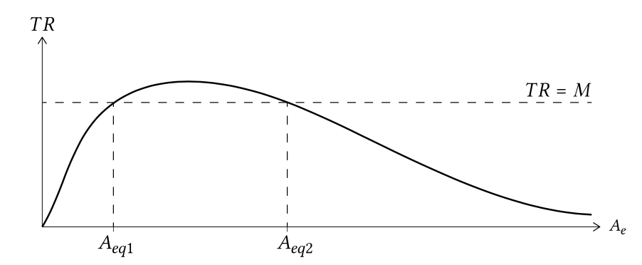
The shapes of the functions, which are independent for realistic values of the parameters \(k\), \(\alpha\) and \(m\), represented by Eqs. \(\ref{eq9.5.2.6}\) and \(\ref{eq9.5.2.7}\), are plotted in Fig. 9.23. In general, there will be two values of the cross-sectional area for which the annual mean ebb tidal transport equals the mean annual influx of sediment \(M\) (\(A_{eq1}\) and \(A_{eq2}\)).
For a given inlet situation with a mean annual influx of sediment \(M\), a difficulty in determining the value of \(A_{eq1}\) and \(A_{eq2}\) from Eqs. \(\ref{eq9.5.2.6}\) and \(\ref{eq9.5.2.7}\) is ascertaining the values \(k\), \(n\), \(m\) and \(\alpha\). An elegant way to circumvent ascertaining the parameters was put forward by Van de Kreeke (2004). For inlets at equilibrium and we find from Eqs. \(\ref{eq9.5.2.6}\) and \(\ref{eq9.5.2.7}\):
\[M = k \alpha^m \hat{u}_e^n A_{e}^{m/2}\]
Subsequently, Van de Kreeke substitutes the relationship between the velocity amplitude of a sinusoidal tide \(\hat{u}_{eq}\) and the cross-sectional area \(A_{eq}\) (Eq. \(\ref{eq9.5.2.2}\)). This yields after some algebra:
\[C = \left ( \dfrac{MT^n}{k \alpha^m \pi^n} \right )^{(\tfrac{2}{m - 2n})}\label{eq9.5.2.9}\]
and
\[q = \dfrac{n}{n - m/2}\label{eq9.5.2.10}\]
Equations \(\ref{eq9.5.2.9}\) and \(\ref{eq9.5.2.10}\) imply that for a set of inlets in equilibrium that have the same values of \(M, T, k, \alpha , m\) and \(n\), values of \(C\) and \(q\) theoretically should be the same. It also follows that \(q > 1\), at least under the present assumptions. This means that data sets used to determine the constants \(C\) and \(q\) in Eq. \(\ref{eq9.5.2.1}\) should ideally consist of inlets that show phenomenological similarity (i.e., have similar values for \(k, n , m\) and \(\alpha\) for a given inlet situation with mean annual influx of sediment \(M\)), implying that the datasets should be clustered while ensuring:
- similar wave driven littoral drift;
- similar tide characteristics (form factor, Eq. 4.4.1.1, and amplitude);
- similar grain size and grain density;
- similar shape of the cross-section.
Most of the data sets published do not fulfil these recommendations and should therefore be considered with care (see Stive et al. (2009) for a review of the datasets). The resolution of this issue is important because slightly different values of \(q\) result in significantly variable values for the equilibrium cross-sectional value of the tidal entrance. This may have significant implications in determining the true stable equilibrium entrance cross-sectional area.