
6.4.1: Definitions
- Page ID
- 16349

\( \newcommand{\vecs}[1]{\overset { \scriptstyle \rightharpoonup} {\mathbf{#1}} } \)
\( \newcommand{\vecd}[1]{\overset{-\!-\!\rightharpoonup}{\vphantom{a}\smash {#1}}} \)
\( \newcommand{\dsum}{\displaystyle\sum\limits} \)
\( \newcommand{\dint}{\displaystyle\int\limits} \)
\( \newcommand{\dlim}{\displaystyle\lim\limits} \)
\( \newcommand{\id}{\mathrm{id}}\) \( \newcommand{\Span}{\mathrm{span}}\)
( \newcommand{\kernel}{\mathrm{null}\,}\) \( \newcommand{\range}{\mathrm{range}\,}\)
\( \newcommand{\RealPart}{\mathrm{Re}}\) \( \newcommand{\ImaginaryPart}{\mathrm{Im}}\)
\( \newcommand{\Argument}{\mathrm{Arg}}\) \( \newcommand{\norm}[1]{\| #1 \|}\)
\( \newcommand{\inner}[2]{\langle #1, #2 \rangle}\)
\( \newcommand{\Span}{\mathrm{span}}\)
\( \newcommand{\id}{\mathrm{id}}\)
\( \newcommand{\Span}{\mathrm{span}}\)
\( \newcommand{\kernel}{\mathrm{null}\,}\)
\( \newcommand{\range}{\mathrm{range}\,}\)
\( \newcommand{\RealPart}{\mathrm{Re}}\)
\( \newcommand{\ImaginaryPart}{\mathrm{Im}}\)
\( \newcommand{\Argument}{\mathrm{Arg}}\)
\( \newcommand{\norm}[1]{\| #1 \|}\)
\( \newcommand{\inner}[2]{\langle #1, #2 \rangle}\)
\( \newcommand{\Span}{\mathrm{span}}\) \( \newcommand{\AA}{\unicode[.8,0]{x212B}}\)
\( \newcommand{\vectorA}[1]{\vec{#1}} % arrow\)
\( \newcommand{\vectorAt}[1]{\vec{\text{#1}}} % arrow\)
\( \newcommand{\vectorB}[1]{\overset { \scriptstyle \rightharpoonup} {\mathbf{#1}} } \)
\( \newcommand{\vectorC}[1]{\textbf{#1}} \)
\( \newcommand{\vectorD}[1]{\overrightarrow{#1}} \)
\( \newcommand{\vectorDt}[1]{\overrightarrow{\text{#1}}} \)
\( \newcommand{\vectE}[1]{\overset{-\!-\!\rightharpoonup}{\vphantom{a}\smash{\mathbf {#1}}}} \)
\( \newcommand{\vecs}[1]{\overset { \scriptstyle \rightharpoonup} {\mathbf{#1}} } \)
\(\newcommand{\longvect}{\overrightarrow}\)
\( \newcommand{\vecd}[1]{\overset{-\!-\!\rightharpoonup}{\vphantom{a}\smash {#1}}} \)
\(\newcommand{\avec}{\mathbf a}\) \(\newcommand{\bvec}{\mathbf b}\) \(\newcommand{\cvec}{\mathbf c}\) \(\newcommand{\dvec}{\mathbf d}\) \(\newcommand{\dtil}{\widetilde{\mathbf d}}\) \(\newcommand{\evec}{\mathbf e}\) \(\newcommand{\fvec}{\mathbf f}\) \(\newcommand{\nvec}{\mathbf n}\) \(\newcommand{\pvec}{\mathbf p}\) \(\newcommand{\qvec}{\mathbf q}\) \(\newcommand{\svec}{\mathbf s}\) \(\newcommand{\tvec}{\mathbf t}\) \(\newcommand{\uvec}{\mathbf u}\) \(\newcommand{\vvec}{\mathbf v}\) \(\newcommand{\wvec}{\mathbf w}\) \(\newcommand{\xvec}{\mathbf x}\) \(\newcommand{\yvec}{\mathbf y}\) \(\newcommand{\zvec}{\mathbf z}\) \(\newcommand{\rvec}{\mathbf r}\) \(\newcommand{\mvec}{\mathbf m}\) \(\newcommand{\zerovec}{\mathbf 0}\) \(\newcommand{\onevec}{\mathbf 1}\) \(\newcommand{\real}{\mathbb R}\) \(\newcommand{\twovec}[2]{\left[\begin{array}{r}#1 \\ #2 \end{array}\right]}\) \(\newcommand{\ctwovec}[2]{\left[\begin{array}{c}#1 \\ #2 \end{array}\right]}\) \(\newcommand{\threevec}[3]{\left[\begin{array}{r}#1 \\ #2 \\ #3 \end{array}\right]}\) \(\newcommand{\cthreevec}[3]{\left[\begin{array}{c}#1 \\ #2 \\ #3 \end{array}\right]}\) \(\newcommand{\fourvec}[4]{\left[\begin{array}{r}#1 \\ #2 \\ #3 \\ #4 \end{array}\right]}\) \(\newcommand{\cfourvec}[4]{\left[\begin{array}{c}#1 \\ #2 \\ #3 \\ #4 \end{array}\right]}\) \(\newcommand{\fivevec}[5]{\left[\begin{array}{r}#1 \\ #2 \\ #3 \\ #4 \\ #5 \\ \end{array}\right]}\) \(\newcommand{\cfivevec}[5]{\left[\begin{array}{c}#1 \\ #2 \\ #3 \\ #4 \\ #5 \\ \end{array}\right]}\) \(\newcommand{\mattwo}[4]{\left[\begin{array}{rr}#1 \amp #2 \\ #3 \amp #4 \\ \end{array}\right]}\) \(\newcommand{\laspan}[1]{\text{Span}\{#1\}}\) \(\newcommand{\bcal}{\cal B}\) \(\newcommand{\ccal}{\cal C}\) \(\newcommand{\scal}{\cal S}\) \(\newcommand{\wcal}{\cal W}\) \(\newcommand{\ecal}{\cal E}\) \(\newcommand{\coords}[2]{\left\{#1\right\}_{#2}}\) \(\newcommand{\gray}[1]{\color{gray}{#1}}\) \(\newcommand{\lgray}[1]{\color{lightgray}{#1}}\) \(\newcommand{\rank}{\operatorname{rank}}\) \(\newcommand{\row}{\text{Row}}\) \(\newcommand{\col}{\text{Col}}\) \(\renewcommand{\row}{\text{Row}}\) \(\newcommand{\nul}{\text{Nul}}\) \(\newcommand{\var}{\text{Var}}\) \(\newcommand{\corr}{\text{corr}}\) \(\newcommand{\len}[1]{\left|#1\right|}\) \(\newcommand{\bbar}{\overline{\bvec}}\) \(\newcommand{\bhat}{\widehat{\bvec}}\) \(\newcommand{\bperp}{\bvec^\perp}\) \(\newcommand{\xhat}{\widehat{\xvec}}\) \(\newcommand{\vhat}{\widehat{\vvec}}\) \(\newcommand{\uhat}{\widehat{\uvec}}\) \(\newcommand{\what}{\widehat{\wvec}}\) \(\newcommand{\Sighat}{\widehat{\Sigma}}\) \(\newcommand{\lt}{<}\) \(\newcommand{\gt}{>}\) \(\newcommand{\amp}{&}\) \(\definecolor{fillinmathshade}{gray}{0.9}\)Sediment transport can be defined as the movement of sediment particles over a certain period of time through a well-defined plane. The vertical extent of such a plane is generally from the bed to the water level. In the horizontal direction the plane may extend from the edge of the surf zone to the water line. In that case the total wave-induced longshore transport integrated over the surf zone is considered. Often however, the transport rates are expressed per metre width.
Since coastal engineers are interested in volumes of accretion and erosion, it is common practice to express the sediment transport rates \(S\) in \(m^3/s/m\) (volumes of sand per second per metre width). These sediment volumes may be expressed in terms of volumes of solid grains. Other sediment transport formulas directly yield the deposited volumes of sand (per second and metre width). Deposited volumes of sand include the pores between the grains and are a factor \(1/(1 - p)\) larger than the volumes of solid grains (see Sect. 6.2.2). In the mass balance Eq. 1.5.2.1, it was assumed that the volumetric sediment transport rates include the pores. If transport rates of solid grains are considered instead, the mass balance reads (with zero local gains or losses):
\[(1 - p) \dfrac{\partial z_b}{\partial t} + \dfrac{\partial S_x}{\partial x} + \dfrac{\partial S_y}{\partial y} = 0\]
where:
| \(z_b (x, t)\) | bed leevel above a certain horizontal datum | \(m\) |
| \(S_x (x, y, t)\) | sediment transport rate in the \(x\)-direction (volume of solid grains per second and per m width) | \(m^3/m/s\) |
| \(S_y (x, y, t)\) | transport rate in the \(y\)-direction | \(m^3/m/s\) |
| \(p\) | porosity | - |
Instead of volumetric transport rates, sometimes mass transport rates are given. This generally does not concern the dry mass of the sediment (with density \(\rho_s\)), but the immersed (underwater) mass of the sediment. The relation between the volumetric transport rate \(S\) (including pores) and the immersed mass transport rate \(I_m\) is:
\[I_m = (\rho_s - \rho)(1 - p) S\]
where:
| \(I_m\) | immersed mass transport rate | \(kg/m/s\) |
| \(S\) | volume transport rates of deposited material | \(m^3/m/s\) |
Other transport formulations are expressed in terms of immersed weight \(I = gI_m\).
The above mentioned transport rates can be instantaneous transport rates, but also transport rates averaged over more hydrodynamic conditions (a wave group, a storm, a year). The latter is of most interest to coastal engineers.
Bed load versus suspended load
Different transport modes can be distinguished:
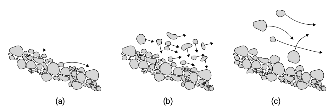
Bed load transport the transport of sediment particles in a thin layer close to the bed. The particles are in more or less continuous contact with the bed. Bed load transport at low shear stresses is shown in Fig. 6.6a. At higher shear stresses, an entire layer of sediment is moving on a plane bed (Fig. 6.6b). This is called sheet flow and is often considered as bed load, since grain-grain interactions play a role.
Suspended load transport the transport of particles suspended in the water without any contact with the bed. The particles are supported by turbulent diffusive forces. Figure 6.6c shows this transport mode.
The sum of bed load and suspended load is called total load. In addition, a third category exists that is named wash load. Wash load consists of very fine particles that will only settle in still water and that are not found in the bed. Since these particles do not contribute to bed level changes, wash load is not taken into account into the total load transport.
Bed-load transport at low shear stresses
As soon as the bed shear stress exceeds a critical value (Shields parameter between 0.03 and 0.06, see Sect. 6.3), sediment particles start rolling or sliding over the bed. If the bed shear stress increases further, the sediment particles move across the bed by making small jumps, which are called saltations. As long as the jump lengths of the saltations are limited to say a few times the particle diameter, this type of motion is considered as a part of the bed load transport. Close to initiation of motion the bed remains flat, but for somewhat larger bed shear stresses the bed load occurs primarily via the migration of small-scale bed forms. When the jumps become larger, the particles loose the contact with the bottom and become suspended.
Sheet-flow transport
At higher shear stresses (Shields parameters higher than about 0.8-1.0), the particles closer to the bed start moving in multiple layers, instead of rolling and jumping in a single layer. In a wave tunnel with reversing flow (see Fig. 6.8), this process can be observed very clearly; the top layer of the bed moves back and forth as a sheet of sand over a flat immobile bed. If the thickness of the sheet-flow layer is defined as the distance between the non-moving bed and the level where the time-averaged sediment concentration becomes lower than a volume concentration of 8 vol.% (see Dohmen-Janssen et al., 2001), the thickness of the sheet-flow layer is in the order of centimetres. For 8 vol.% the distance between particles is on average equal to the grain diameter. This means that intergranular forces and grain-water interactions are important. Bagnold (1956) defined bed load as that part of the total load that is supported by intergranular forces. According to this definition sheet-flow transport can be considered as bed load transport at high shear stresses.
Suspended load transport
Above the bed load layer or sheet-flow layer, sediment may be in suspension. Particles in suspension do not immediately return to the bed under the influence of their settling velocity, but are kept in suspension by fluid turbulence. Suspended particles present in a certain vertical plane can be assumed to move horizontally across the plane with the water particles and thus at the speed of the water particles. The particles are suspended in the flow at relatively low concentrations (less than 1 vol.%), so that intergranular forces are not important.
As mentioned above, in the sheet-flow regime (Shields parameters above 0.8-1.0) an entire layer of sediment is moving on a plane bed. Because the bed is plane, the as- sumption seems reasonable that the suspended load above the sheet-flow layer is supported by fluid turbulence (or in other words: that the vertical transport of sediment is governed by turbulent diffusive processes). Suspended transport supported by fluid turbulence is further treated in Sect. 6.6.
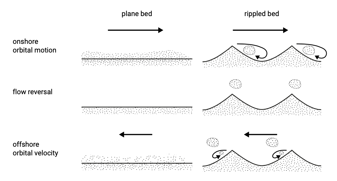
At lower Shields parameters however (below 0.8–1.0), the bed will not remain plane. Instead smaller and larger bed forms occur under the influence of currents and the wave orbital motion. Orbital ripples have a length in the order of the free stream orbital velocity amplitude \(\hat{u}_0\) (see Sect. 5.4.3 and Eq. 5.4.3.1), whereas anorbital ripples are much smaller and scale with the grain size. In the case of a rippled bed, the bed roughness is related to the ripple geometry instead of to the grain diameter as was the case for a plane bed. Further, the flow separates behind the ripple crest and an organised pattern of vortices is formed near the bed (see Fig. 6.7).
These vortices are capable of bringing large amounts of sediment into suspension. The timing of these suspension events within the wave cycle is crucial for the magnitude (and the direction, see Sect. 6.6.1 and Intermezzo 6.1) of the resulting wave-averaged sediment transport. Whereas in the plane bed case, it is normally assumed that turbulent diffusive forces keep the sediments in suspension, for a rippled bed, a different approach should be taken because the upward transport of sediment is now the result of an organised motion. This complicates the computation of \(c(z, t)\) as well as of \(v(z, t)\) considerably and is not explicitly considered in these lecture notes.
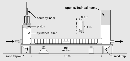
Figure 6.8: Schematic representation of the Large Oscillating Water Tunnel (LOWT)(LOWT) used in the Netherlands to study intra-wave sediment transport phenomena under controlled simulated wave conditions at full scale. The system basically consists of a vertical U-tube with one open leg. The other leg is provided with a piston. At the bottom of the test section a sediment bed may be installed. The generated oscillatory flow is purely horizontal; as opposed to the case of progressive waves, vertical velocities and horizontal gradients, and thus wave-induced streaming, are absent.
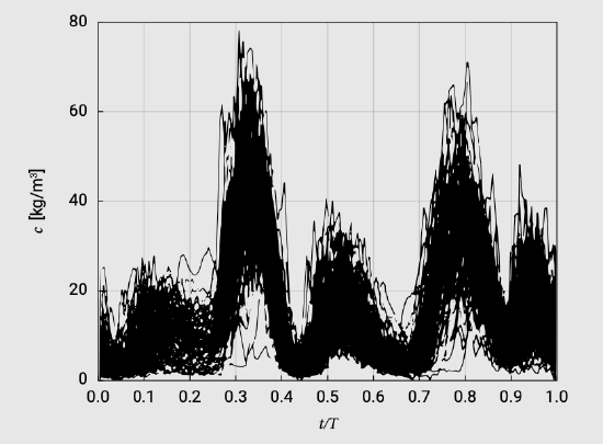
Figure 6.9: Sediment concentrations as a function of time (99 individual records) (Bosman, 1982). On the \(x\)-axis: time \(t\) relative to wave period \(T\). On the \(y\)-axis: sediment concentration in \(kg/m^3 (= g/l)\). Sinusoidal water motion \(\hat{u}_0 = 0.3\ m/s\) and \(T = 1\ s\), measured at ripple crest position.
In a coastal environment both the velocity and the concentration exhibit large variations within a wave period. Unfortunately, insight regarding \(c(z, t)\) especially is very poor. Even in a relatively simple laboratory case of a wave tunnel (Fig. 6.8), the relation between flow kinematics and sediment concentration is far from unambiguous. This can be seen from Fig. 6.9 where nearly a hundred different records of \(c(t)\) are shown, all measured at a constant near-bed elevation and under identical regular wave conditions. The scatter in the measuring results is very large. Nevertheless, we can see the following qualitative behaviour:
- A peak in the sediment concentration just after the maximum onshore and offshore velocity (\(t/T = 0.25\));
- Two secondary peaks in sediment concentration just after flow reversal (associated with vortices developing over a rippled bed).
The behaviour of \(c(z, t)\) in irregular progressive and breaking waves is even less well understood and very difficult to model with a reasonable accuracy. This has serious implications for the accuracy of calculations of the intra-wave sediment flux \(c(z, t) \cdot u(z, t)\). Besides, due to the oscillatory behaviour of \(u(z, t)\), its average value is close to zero, making the computations very sensitive to errors.
Measurements in wave flumes (as opposed to tunnels) show the presence of suspended sediment particles from the bed up to the (instantaneous) water surface. The largest concentrations are found close to the bed where the diffusivity is large due to ripple-generated eddies. Further away from the bed the sediment concentrations decrease rapidly because the eddies dissolve rather rapidly travelling upwards.