21.8: Natural Oscillations

The 30-year-average climate is called the normal climate. Any shorter-term (e.g., monthly) average weather that differs or varies from the climate norm is called an anomaly. Natural climate “oscillations” are recurring, multi-year anomalies with irregular amplitude and period, and hence are not true oscillations (see the INFO Box).

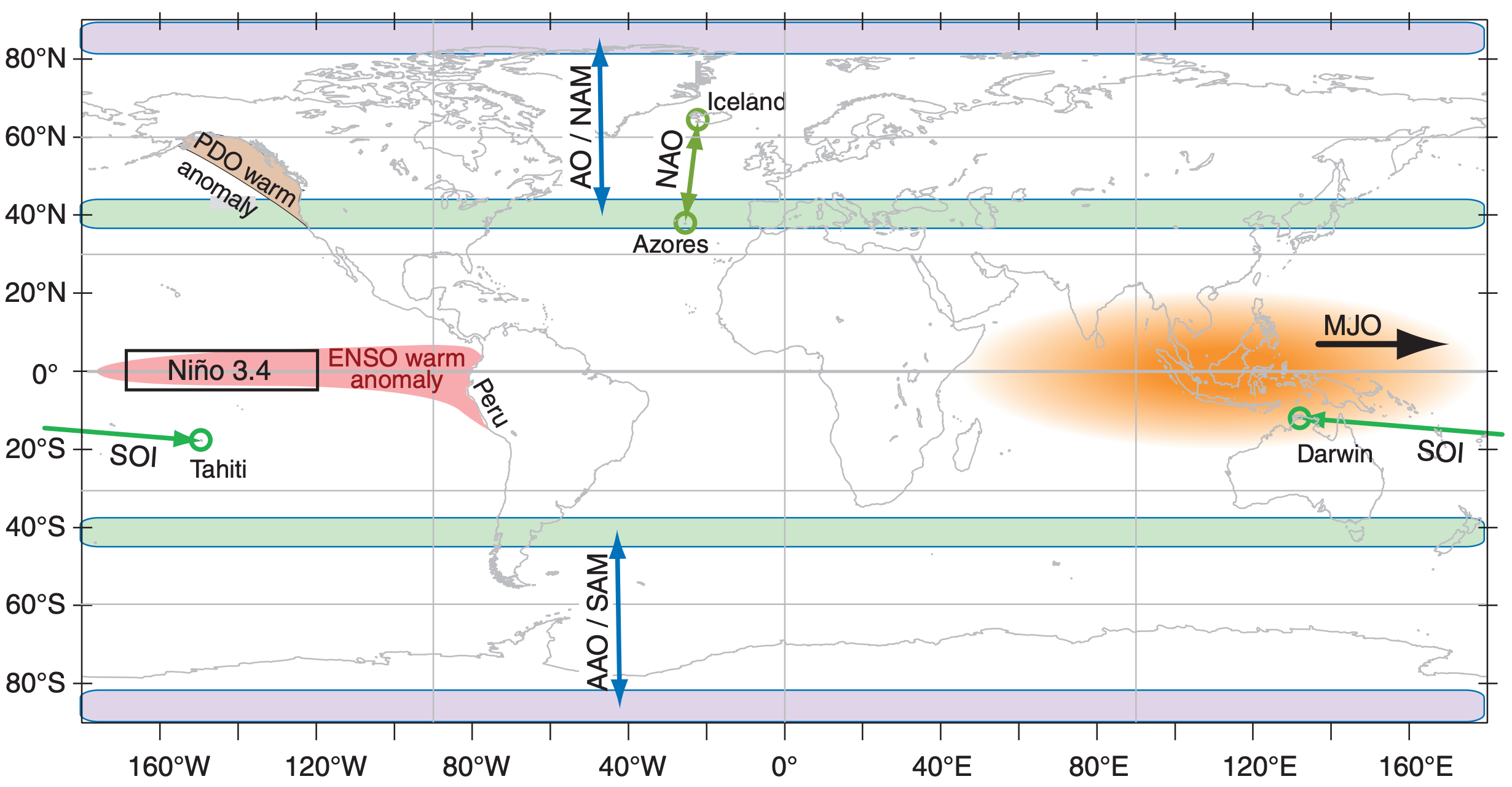
Table 21-7 lists some of these oscillations and their major characteristics. Although each oscillation is associated with, or defined by, a location or place on Earth (Fig. 21.26), most of these oscillations affect climate over the whole world. At the defining place(s), a combination of key weather variables is used to define an “index”, which is the varying climate signal. Fig. 21.27 shows some of these oscillation indices.

Table 21-7. Climate oscillations. SST = sea-surface temperature, SLP = sea-level pressure.

Name	Period (yr)	Key Place	Key Variable
El Niño (EN)	2 to 7	Tropical E. Pacific	SST
Southern Oscillation (SO)	2 to 7	Tropical Pacific	SLP
Pacific Decadal Oscillation (PDO)	20 to 30	Extratrop. NE Pacific	SST
North Atlantic Oscillation (NAO)	variable	Extratrop. N. Atlantic	SLP
Arctic Oscillation (AO)	variable	N. half of N. hem.	SLP
Madden-Julian Oscillation (MJO)	30 to 60 days	Tropical Indian & Pacific	Convective Precipitation

INFO • What is an Oscillation?

Oscillations are regular, repeated variations of a measurable quantity such as temperature (T) in space x and/or time t. They can be described by sine waves:

\[T=A \cdot \sin \left[C \cdot\left(t-t_{o}\right) / \tau\right\]

where A is a constant amplitude (signal strength), \(\tau\) is a constant period (duration one oscillation), t_o is a constant phase shift (the time delay after t = 0 for the signal to first have a positive value), and C is 2π radians or 360° (depending on your calculator).

True oscillations are deterministic — the signal T can be predicted exactly for any time in the future. The climate “oscillations” discussed here are not deterministic, cannot be predicted far in the future, and do not have constant amplitude, period, or phase.

Figure 21.26 Places and key variables that define some climate oscillations. Acronyms are defined in the text.

21.8.1. El Niño - Southern Oscillation (ENSO)

El Niño (La Niña) occurs when the tropical sea-surface temperature (SST) in the central and eastern Pacific ocean is warmer (cooler) than the multi-decadal climate average.

The El Niño index plotted in Fig. 21.27a is the Pacific SST anomaly in the tropics (Niño region 3.4, averaged within ±5° latitude of the equator, between 170 - 120°West) minus the Pacific SST anomaly outside the tropics (averaged over more poleward latitudes). Alternative El Niño indices are also useful.

Figure 21.27 Natural oscillations of some climate indices.

(a) El Niño 3.4 index, based on average sea-surface temperature (SST) anomalies ∆T. [Data courtesy of https://www.esrl.noaa.gov/ psd/enso/dashboard.html.]

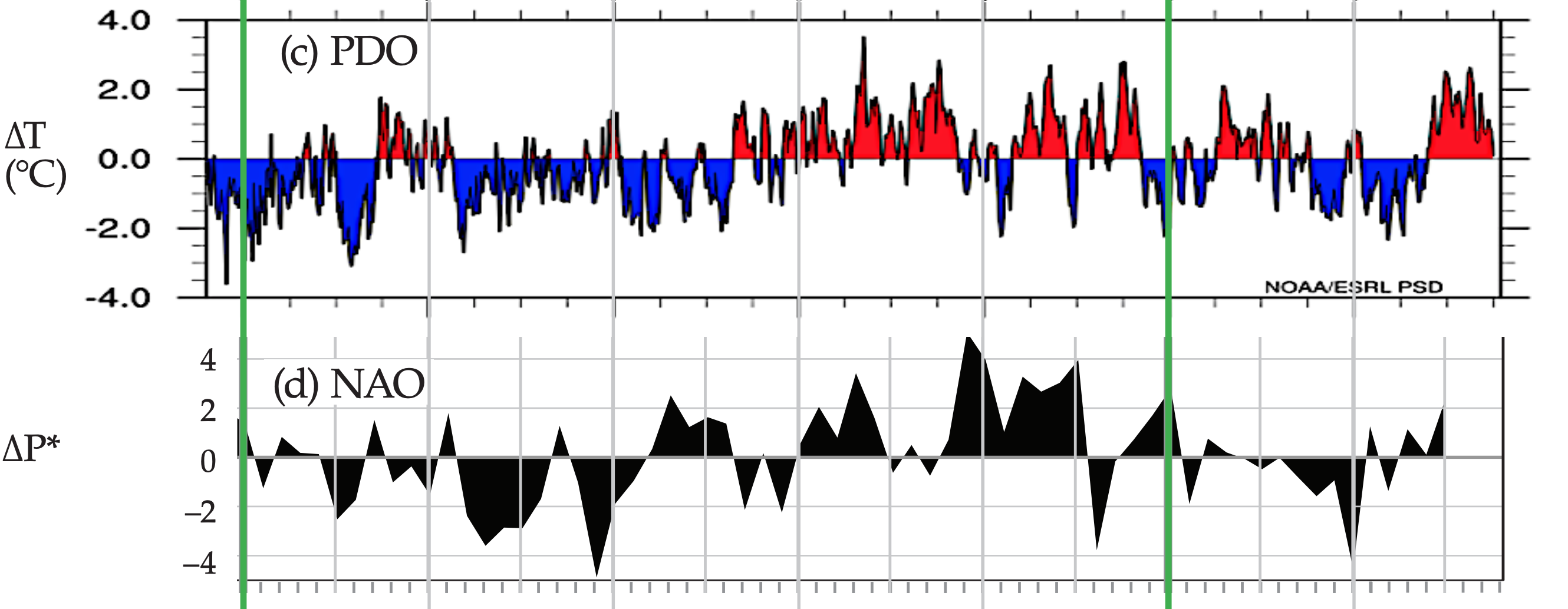
(c) Pacific Decadal Oscillation (PDO) index, based on the leading principal component for monthly Pacific SST variability north of 20°N latitude after global mean SST is removed. [Data courtesy of https://www.esrl.noaa.gov/psd/enso/dashboard.html.]

(d) North Atlantic Oscillation (NAO) index, based on the difference of normalized SLP (defined on p 824): ∆P* = P*_Azores – P*_Iceland for winter (Dec - Mar) [Data courtesy of Jim Hurrell, NCAR/CGD/CAS.]

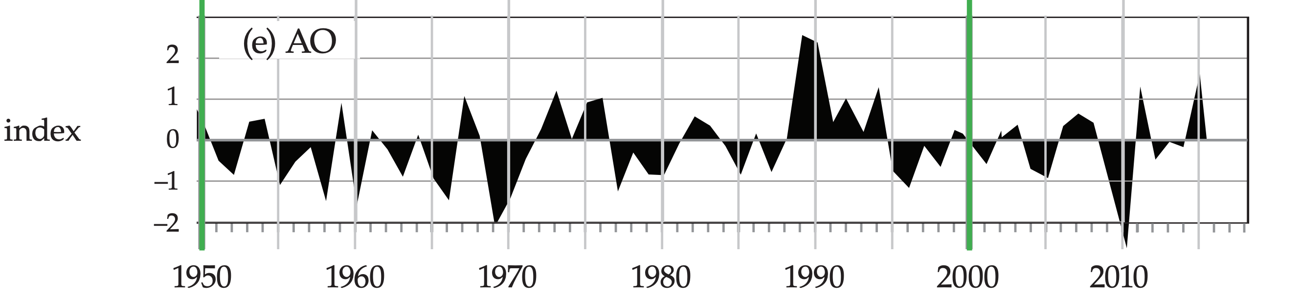
(e) Arctic Oscillation (AO) index, based on the leading principal component of winter SLP in the N. Hemisphere for winter (Jan-Mar) [Data courtesy of Todd Mitchell of the Univ. of Washington Joint Inst. for Study of the Atmos. & Ocean (US JISAO).]

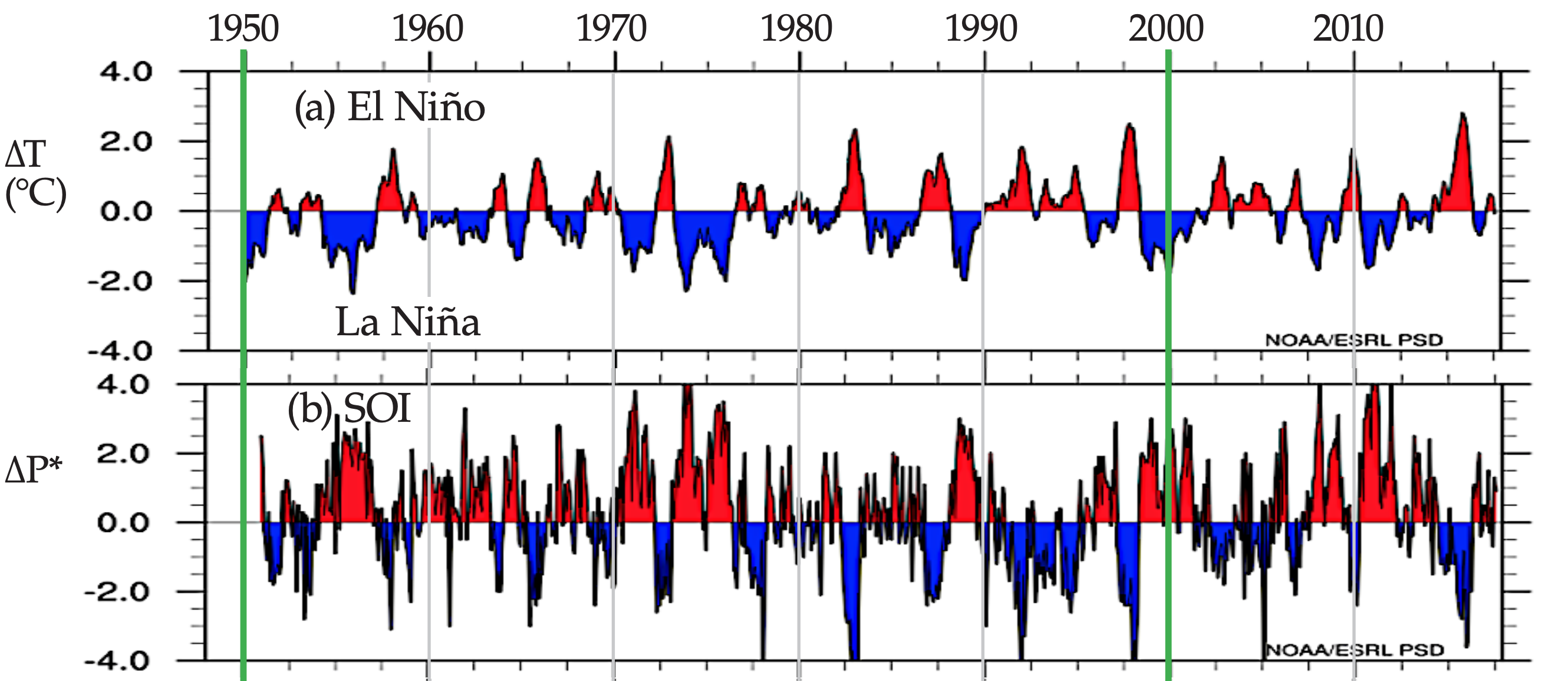
The Southern Oscillation refers to a change in sign of the east-west atmospheric pressure gradient across the tropical Pacific and Indian Oceans. One indicator of this pressure gradient is the sea-level pressure difference between Tahiti (an island in the central equatorial Pacific, Fig. 21.26) and Darwin, Australia (western Pacific). This indicator (∆P = P_Tahiti – P_Darwin) is called the Southern Oscillation Index (SOI).

The SOI, plotted in Fig. 21.27b, varies oppositely to (i.e., is negatively correlated with) the El Niño index (Fig. 21.27a). The reason for this correlation is that El Niño (EN) and the Southern Oscillation (SO) are, respectively, the ocean and atmospheric signals of the same coupled phenomenon, abbreviated as ENSO.

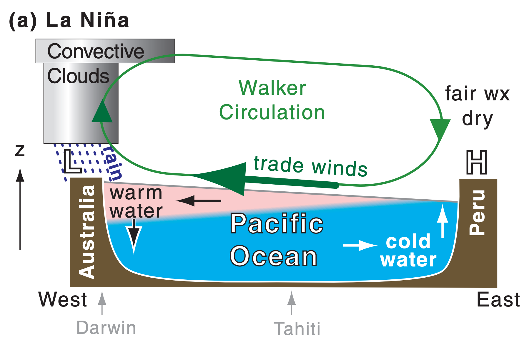
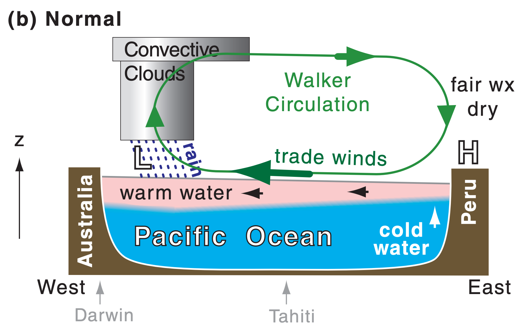
During normal and La Niña conditions, the east-to-west decrease in air pressure drives the easterly trade winds, which drag much of the warm ocean-surface waters to the west side of the Pacific basin (Fig. 21.28a). The trade winds are part of the Walker Circulation, which includes cloudy rainy updrafts over the warm SST anomaly in the western tropical Pacific, a return flow aloft, and fair-weather (“fair wx”) dry downdrafts. Heavy rain can fall over Australia. Other changes are felt around the world, including cool winters over northern N. America, with drier warmer winters over the southern USA.

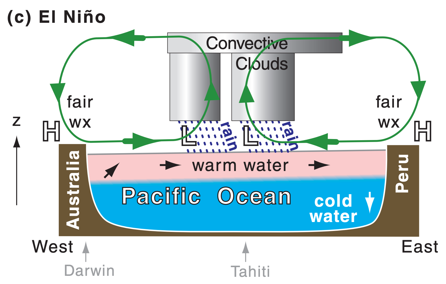
During El Niño, this pressure gradient breaks down, causing the trade winds to fail, and allowing anomalously warm western Pacific waters to return to the eastern Pacific (Fig. 21.28c). Thunderstorms and rain tend to be strongest over the region of warmest SST. As the SST anomaly shifts eastward, droughts (allowing wild fires) occur in Australia, and heavy rains (causing floods and landslides) occur in Peru. Other changes are felt around the world, including warm winters over northern N. America and cool, wet winters over southern N. America.

Figure 21.28 Processes that drive ENSO. (a) La Niña conditions, where cold upwelling nutrient-rich water off the coast of Peru enables increases in fish populations. Also, cool equatorial water upwells near the central Pacific. Strong trade winds. (b) Normal conditions, with modest trade winds. (c) El Niño conditions, associated with a warm-water anomaly in the eastern Pacific, and a decline in fish stocks there. H and L indicate centers of high and low atmospheric pressure, respectively.

21.8.2. Pacific Decadal Oscillation (PDO)

The PDO is a 20- to 30-year variation in the extratropical SST (Fig. 21.27c) near the American coast in the NE Pacific. It has a warm or positive phase (i.e., warm in the key place sketched in Fig. 21.26) and a cool or negative phase. The PDO signal is found using a statistical method called principal component analysis (PCA, also called empirical orthogonal function analysis, EOF; see the INFO box on the next three pages.)

The PDO affects weather in northwestern North America as far east as the Great Lakes, and affects the salmon production between Alaska and the Pacific Northwest USA. There is some debate among scientists whether the PDO is a statistical artifact associated with the ENSO signal.

INFO • PCA and EOF

Principal Component Analysis (PCA) and Empirical Orthogonal Function (EOF) analysis are two names for the same statistical analysis procedure. They are a form of data reduction designed to tease out dominant patterns that naturally occur in the data. Contrast that with Fourier analysis, which projects the data onto sine waves regardless of whether the data naturally exhibits wavy patterns or not.

You can use a spreadsheet for most of the calculations, as is illustrated here with a contrived example.

1) The Meteorological Data to be Analyzed

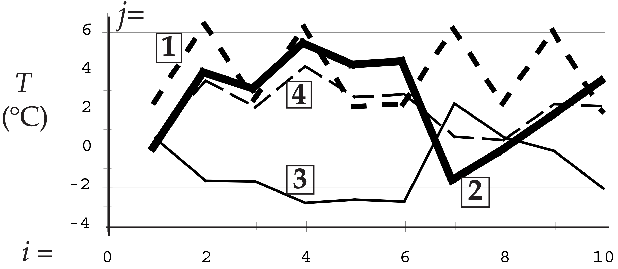
Suppose you have air temperature T measurements from different locations over the North Pacific Ocean. Although PCA works for any number of locations, we will use just 4 locations for simplicity:

Fig. 21.a. Locations for weather data.

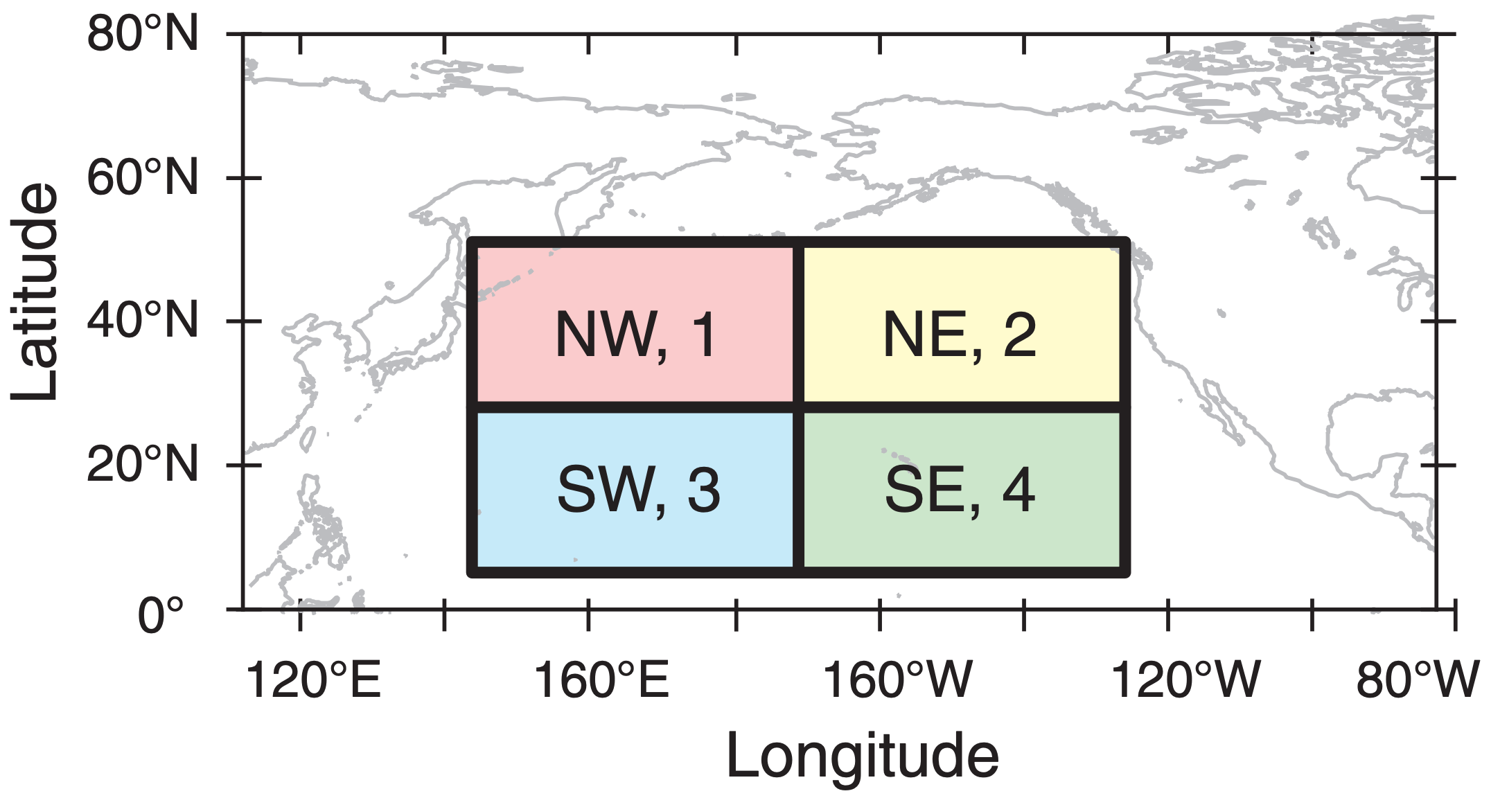
These 4 locations might have place names such as Northwest quadrant, Northeast quadrant, etc., but we will index them by number: j = 1 to 4. You can number your locations in any order.

For each location, suppose you have annual average temperature for N = 10 years, so your raw input data on a spreadsheet might look this:

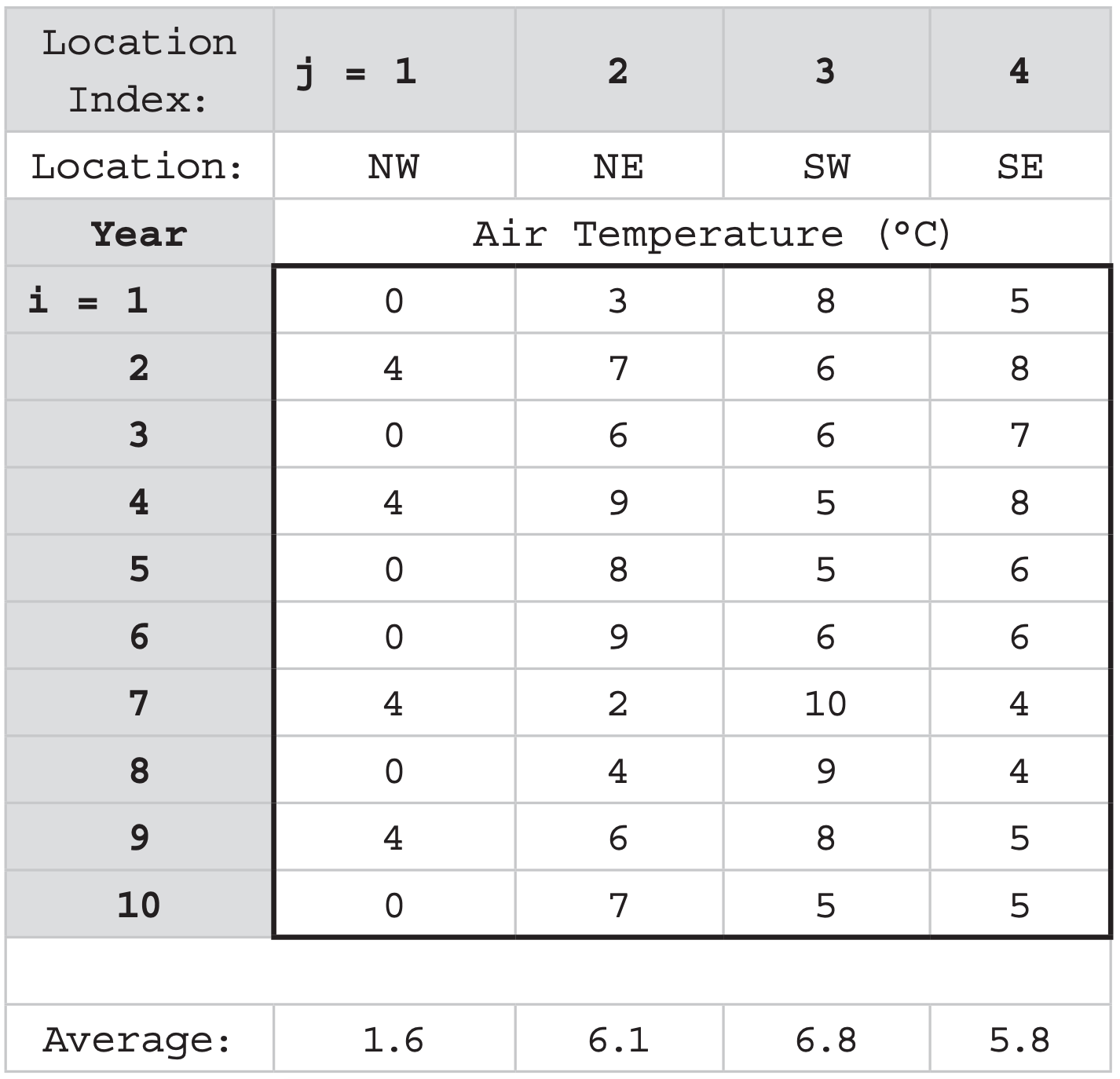
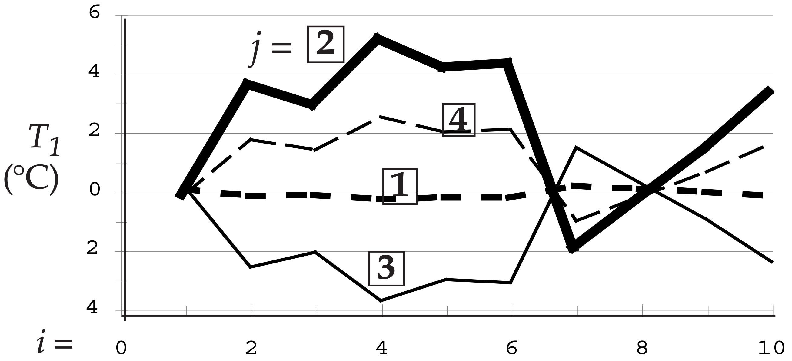
These meteorological data are plotted below:

Fig. 21.b. Graphs of raw data at each of 4 locations, where numbers in boxes indicate the j index for each line, and i = 1 to 10 years.

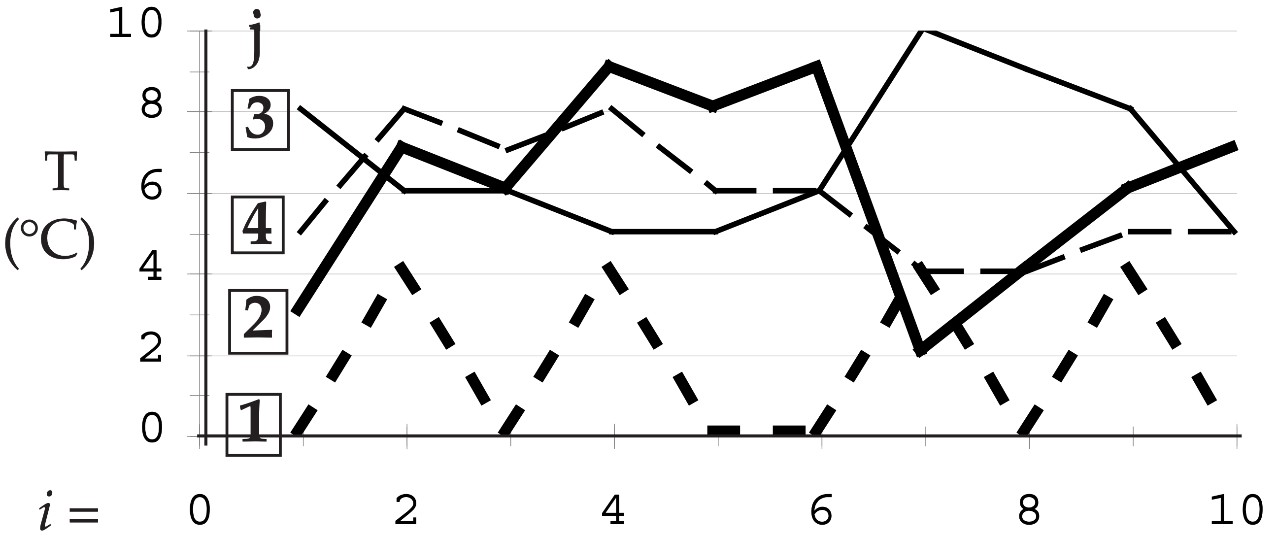
Looking at this data by eye, we see that location 2 has a strong signal. Location 4 varies somewhat similarly to 2 (i.e., has positive correlation); location 3 varies somewhat oppositely (negative correlation). Location 1 looks uncorrelated with the others.

2) Preliminary Statistical Computations

Next, use your spreadsheet to find the average temperature at each location (shown at the bottom of the previous table). Then subtract the average from the individual temperatures at the same locations, to make a table of temperature anomalies T ’:

\begin{align}T_{i}^{\prime}=T_{i}-T_{a v g}\tag{21.48}\end{align}

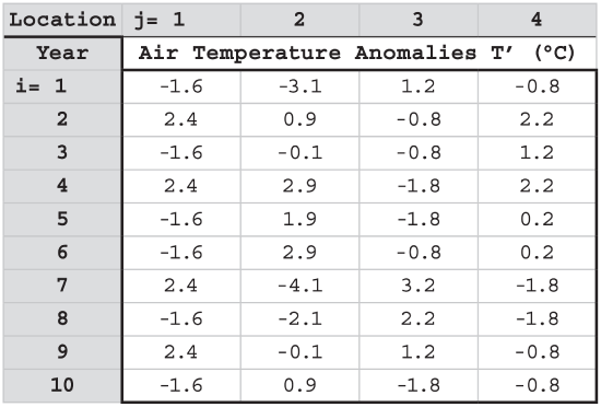
[Check: The average of each T’ column should = 0.]

The covariance between variables A and B is:

\begin{align}\operatorname{covar}(A, B)=\dfrac{1}{N} \sum_{i=1}^{N} A_{i}^{\prime} \cdot B_{i}^{\prime}\tag{21.49}\end{align}

where covar(A,A) is the variance. Use a spreadsheet to compute a table of covariances, where T1 are the temperatures at location j=1, T2 are from location 2, etc.:

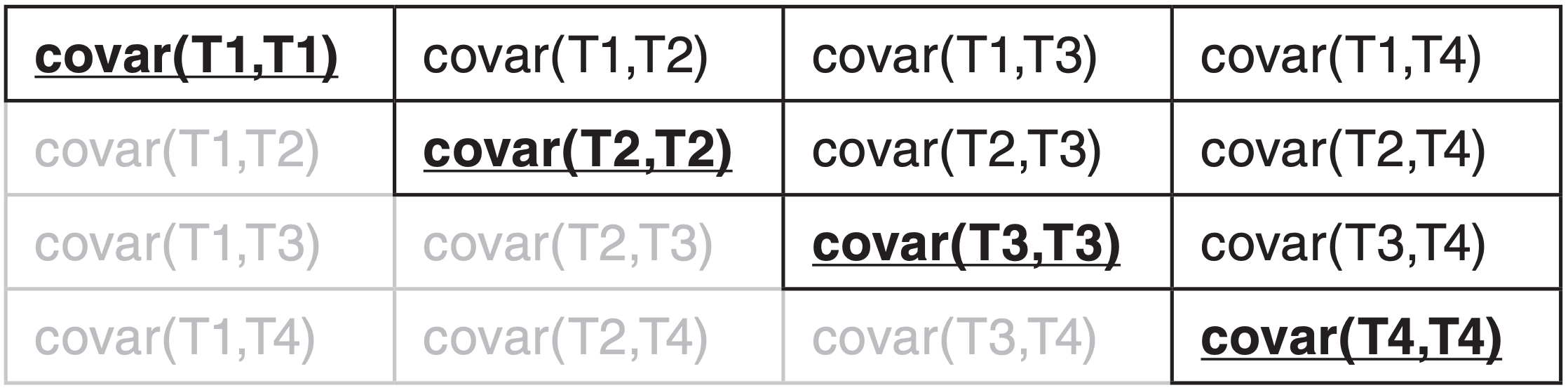
The numbers in that table are symmetric around the main diagonal, so you need to compute the covariances for only the black cells, and then copy the appropriate covariances into the grey cells.

This table is called a covariance matrix. When I did it in a spreadsheet, I got the values below:

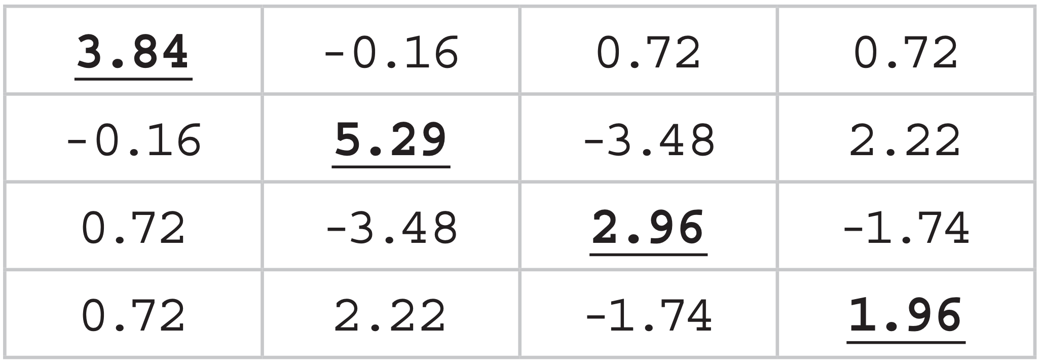
The underlined values along the main diagonal are the variances. The sum of these diagonal elements (known as the trace of the matrix) is a measure of the total variance of our original data (= 14.05 °C²).

3) More Statistical Computations

Next, find the eigenvalues and eigenvectors of the covariance matrix. You cannot do that in most spreadsheets, but other programs can do it for you.

I used a website: http://www.arndt-bruenner.de/mathe/ scripts/engl_eigenwert2.htm where I copied my covariance matrix into the web page, and specified the eigenvectors to have absolute value of 1. It gave back the following info, which I pasted into my spreadsheet. Under each eigenvalue is the corresponding eigenvector.

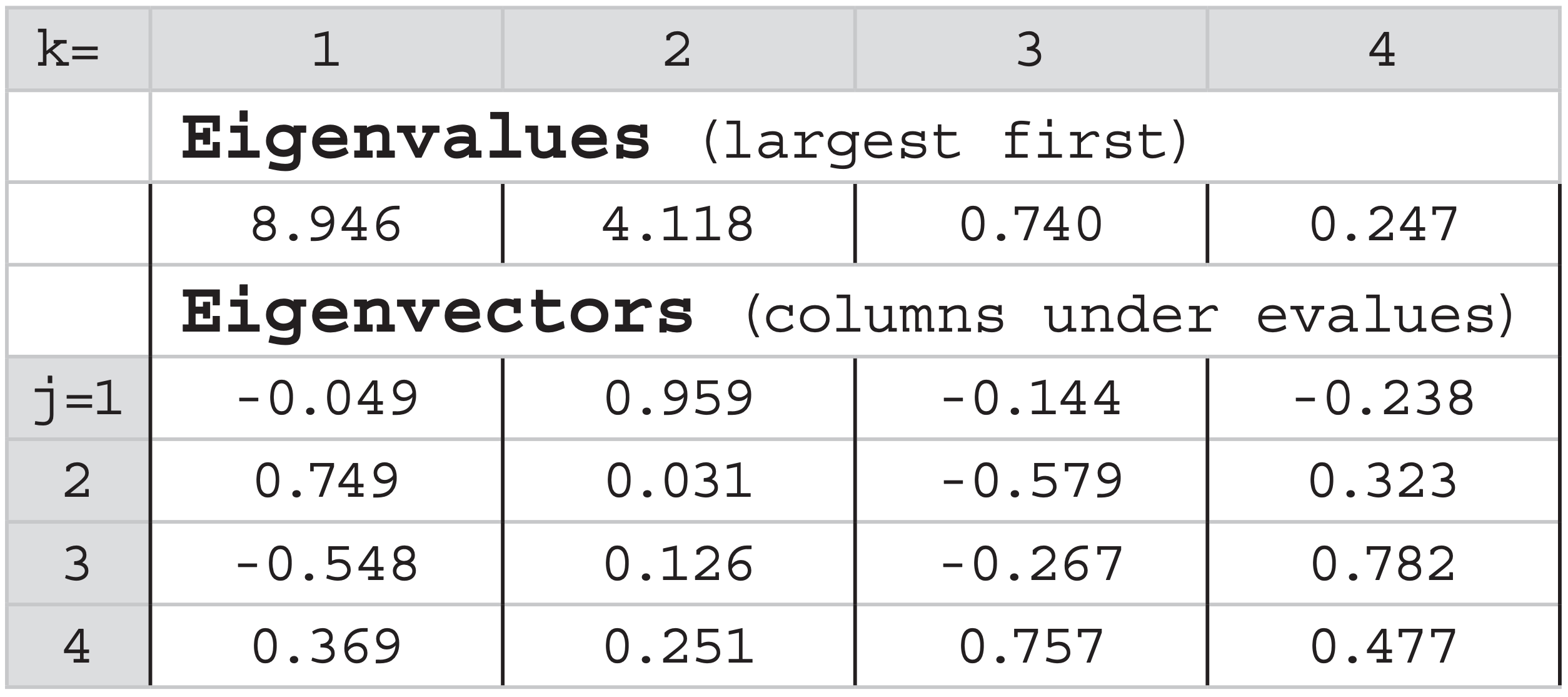
The sum of all eigenvalues = 14.05 °C² = the total variance of the original data. Those eigenvectors with the largest eigenvalues explain the most variance. Eigenvectors are dimensionless.

4) Find the Principal Components

Next, compute the principal components (PCs) — one for each eigenvector (evect). The number of eigenvectors (K = 4 in our case) equals the number of locations (J = 4 in our case).

Each PC will be a column of N numbers (i = 1 to 10 in our case) in our spreadsheet. Compute each of these N numbers in your spreadsheet using:

\begin{align}P C(k, i)=\sum_{j=1}^{J}[e v e c t(k, j) \cdot T(j, i)]\tag{21.50}\end{align}

For each variable (T data; eigenvectors; PCs) used in eq. (21.50), the first index indicates the column and the second indicates the row.

Namely:

• k indicates which PC it is (k = 1 for the first PC, k = 2 for the second PC, up through k = 4 in our case) and also indicates the eigenvector (evect).
• i is the observation index (i = 1 to N, where N = 10 yrs in our case), and indicates the corresponding element in any PC.
• j is the data variable index (1 for NW quadrant, etc.), and indicates an element within each eigenvector.

For example, focus on the first PC (i.e., k = 1; the first column in the table below). The first row (i = 1) is computed as:

PC(1,1) = –0.049·0 + 0.749·3 –0.548·8 + 0.369·5 = –0.29

For the second row (i = 2), it is:

PC(1,2) = –0.049·4 + 0.749·7 –0.548·6 + 0.369·8 = 4.71

Each PC element has the same units as the original data (°C in our case). The resulting PCs are:

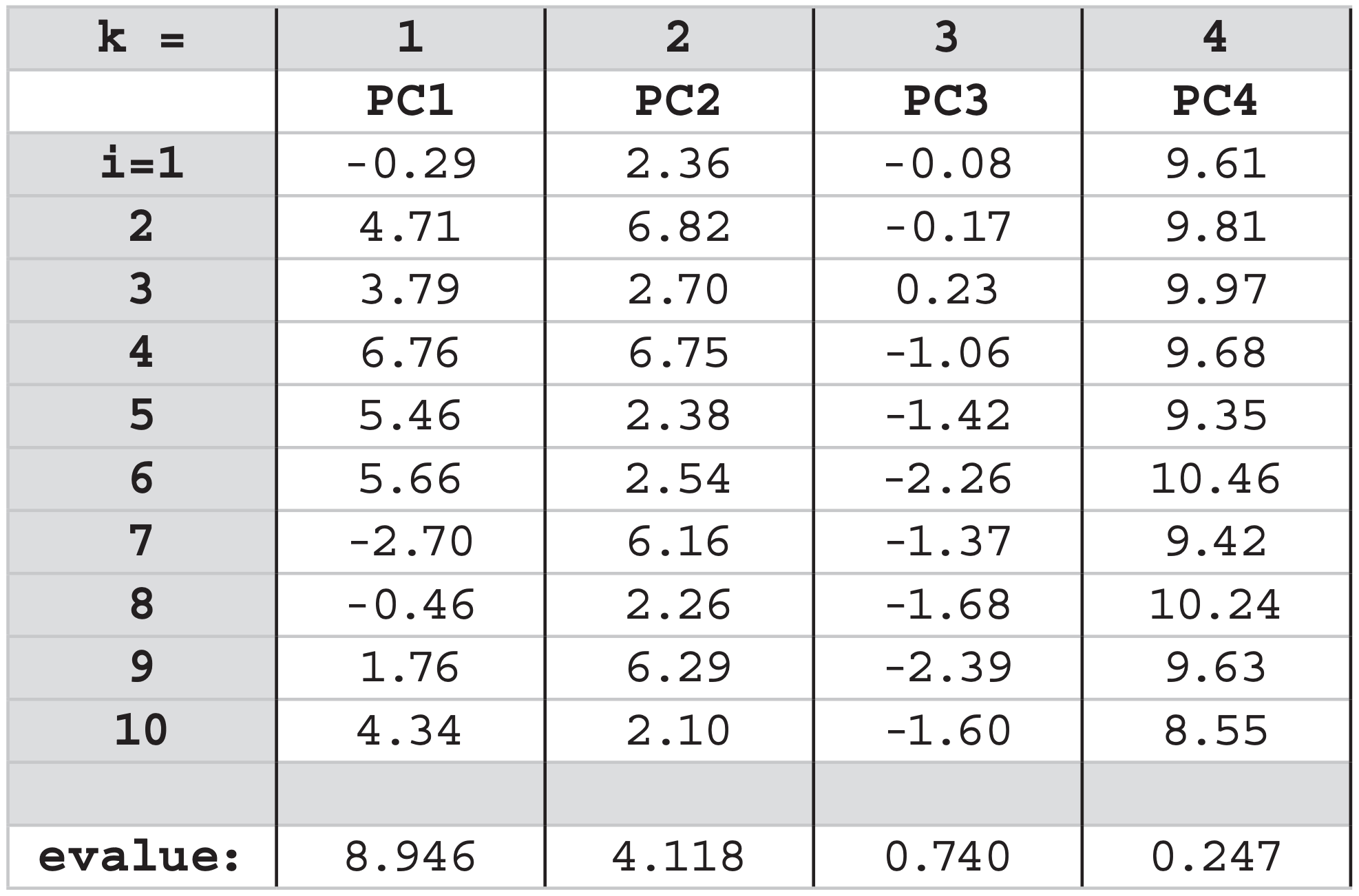
Each PC applies to the whole data set, not just to one location. These PCs, plotted below, are like alternative T data:

Fig. 21.c. PCs, where i = 1 to 10 years.

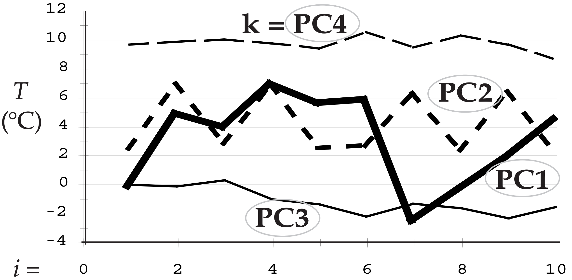
• PC1 captures the dominant pattern that is in the raw data for locations 2, 3, and 4. This 1^st PC explains 8.946/14.05 = 63.7% of the original total variance.
• PC2 captures the oscillation that is in the raw data for location 1. Since location 1 was uncorrelated with the other locations, it couldn’t be captured by PC1, and hence needed its own PC. The 2^nd PC explains 4.118/14.05 = 29.3% of the variance.
• PC3 captures a nearly linear trend in the data.
• PC4 captures a nearly constant offset.

5) Synthesis

Now that we’ve finished computing the PCs, we can see how well each PC explains the original data. Let T_k be an approximation to the original data, re-constructed using only the k^th single principal component. Such reconstruction is known as synthesis.

\begin{align}T_{k}(j, i)=\operatorname{evect}(k, j) \cdot P C(k, i)\tag{21.51}\end{align}

using the same (column, row) notation as before.

For k = 1 (the dominant PC), the reconstructed T₁ data is:

Fig. 21.d. Reconstruction of temperature for each geographic location j = 1 to 4 (boxed numbers), but using only the 1st PC. i = 1 to 10 years.

It is amazing how well just one PC can capture the essence (including positive and negative correlations) of the signal patterns in the raw data.

The spatial pattern associated with PC1 can be represented on a map by the elements of the first eigenvector [namely, the first eigenvector column in section (3) arbitrarily scaled by 100 here & rounded]:

Fig. 21.e. Geographic pattern of influence of PC1.

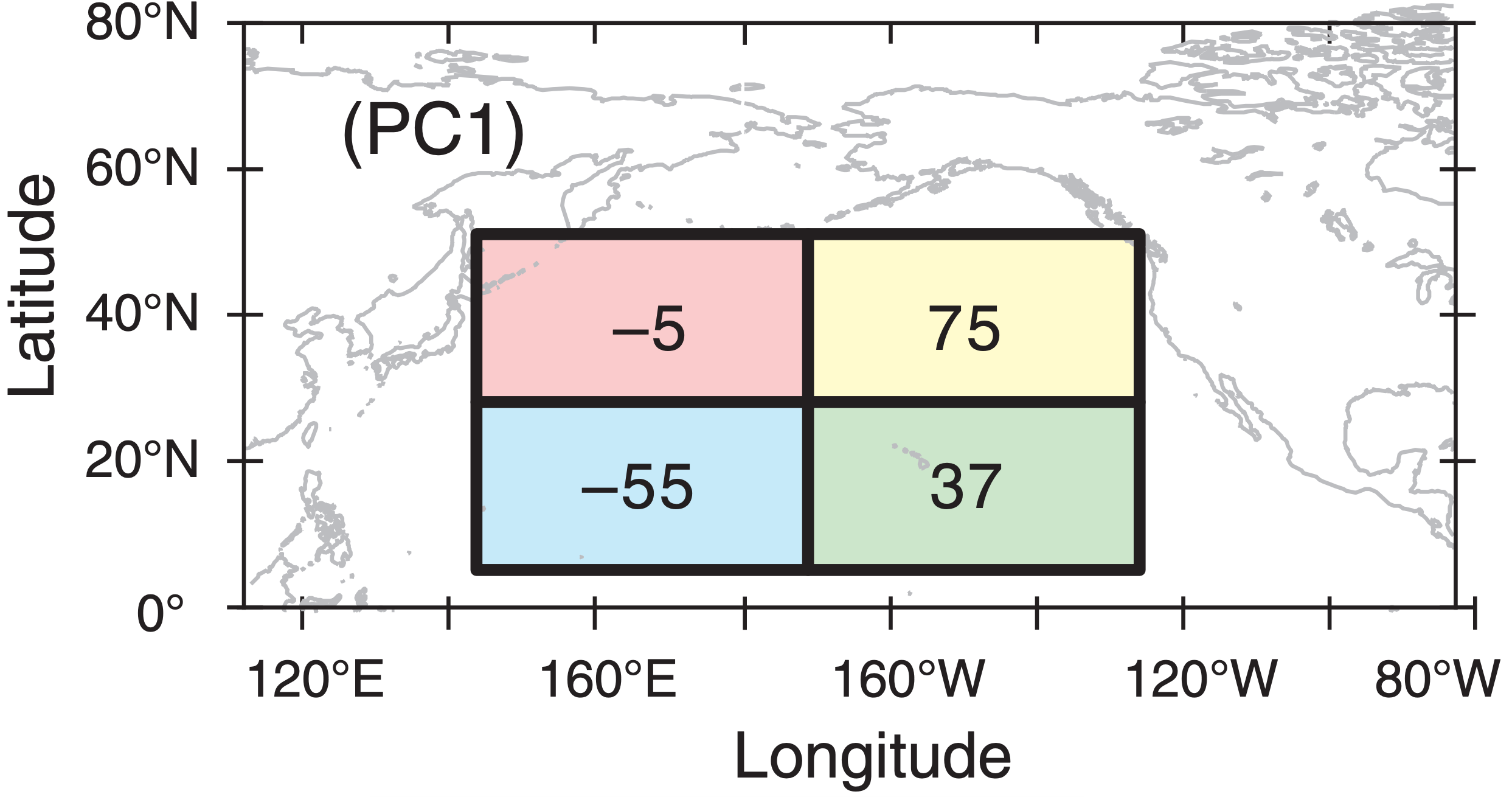
6) Interpretation:

A dominant pattern in the NE quadrant extends in diminished form to the SE quadrant, with the SW quadrant varying oppositely. But this pattern is not experienced very much in the NW quadrant. Similar maps can be created for the other eigenvectors. When data from more than 4 stations are used, you can contour the eigenvector data when plotted on a map.

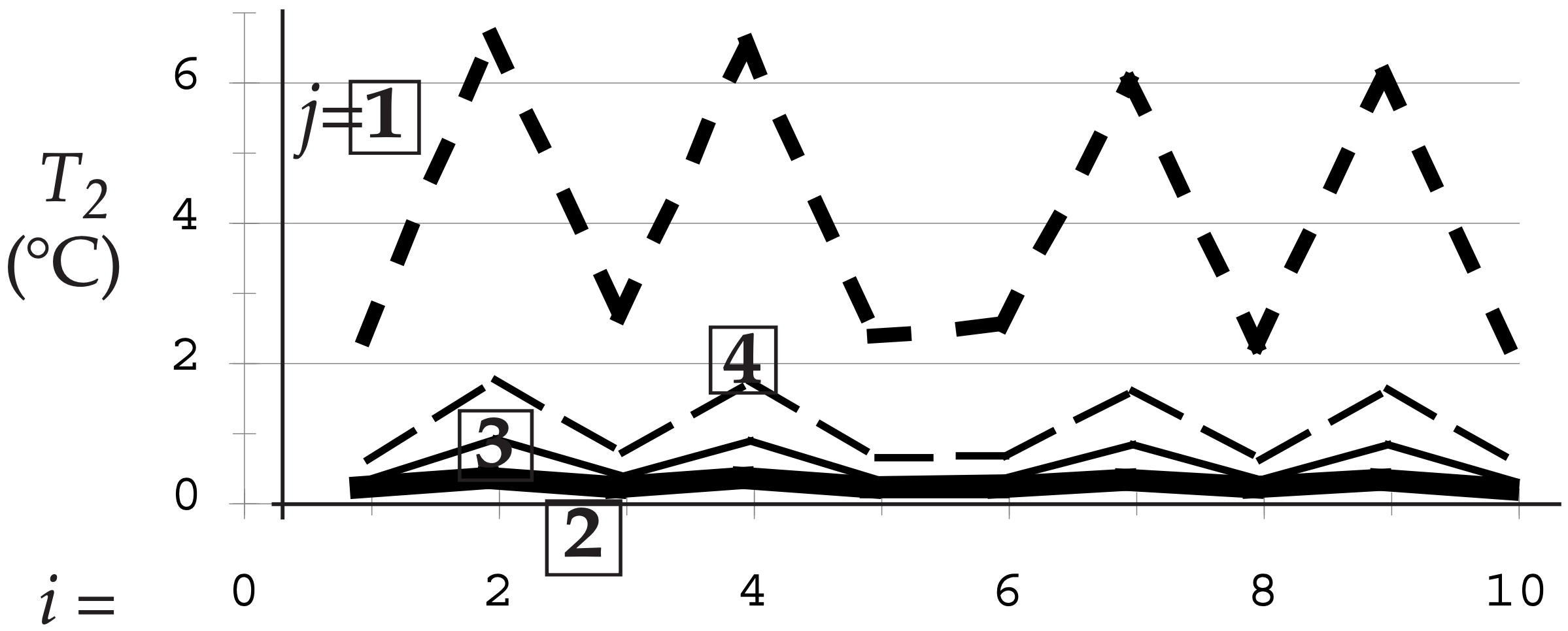
Eq. (21.51) can also be used to partially reconstruct the data based on only PC2 (i.e., k = 2). As shown in Fig. 21.f, you won’t be surprised to find that it almost completely captures the signal in the NW quadrant (j = 1), but doesn’t explain much in the other regions.

Fig. 21.f. Similar to Fig. 21.d, but using only PC2.

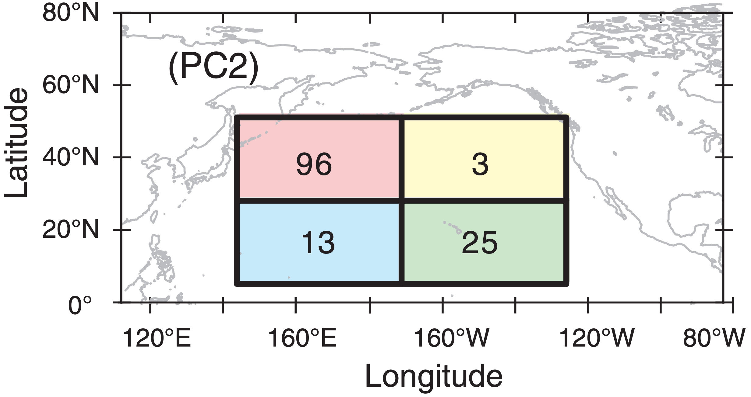
Plotting the elements of the 2^nd eigenvector (from section 3; scaled by 100 and rounded) on a map at their geographic locations:

Fig. 21.g. Geographic pattern of influence of PC2.

7) Data Reduction

Suppose that you compute graphs similar to Figs. 21.d & 21.f for the other PCs, and then add all location 1 curves from each PC. Similarly, add all location 2 curves together, etc. The result would perfectly synthesize the original data as was plotted in Fig. 21.a. Although the last 2 PCs don’t explain much of the variance (fluctuations of the raw data), they are important to get the mean temperature values.

But what happens if you synthesize the temperature data with only the first 2 PCs (see plot below). These first 2 PCs explain 93% of the total variance. Indeed, the graph below captures most of the variation in the original signals that were in Fig. 21.a, including positive, negative, and near-zero correlations. This allows data reduction: We can use only the dominant 2 PCs to explain most of the signals, instead of using all 4 columns of raw data.

Fig. 21.h. Reconstruction of temperature using only the first 2 PCs.

8) Conclusions

For our small data set, the data reduction might not seem like much, but for larger data sets with hundreds of geographic points, this can be an important way to find dominant patterns in noisy data, and to describe these patterns efficiently. For this reason, PCA/EOF is valued by climate researchers.

21.8.3. North Atlantic Oscillation (NAO)

In the General Circulation chapter (Fig. 11.31) we identified an Iceland low and Azores (or Bermuda) high on the map of average sea-level pressure (SLP). The NAO is a variation in the strength of the pressure difference between these two pressure centers (Fig. 21.26).

Greater differences (called the positive phase of the NAO) correspond to stronger north-south pressure gradients that drive stronger west winds in the North Atlantic — causing mid-latitude cyclones and associated precipitation to be steered toward N. Europe. Weaker differences (negative phase) cause weaker westerlies that tend to drive the extratropical cyclones toward southern Europe.

An NAO index is defined as ∆P* = P*_Azores – P*_Iceland, where P* = (P – P_clim)/σ_P is a normalized pressure that measures how many standard-deviations (σ_P) the pressure is from the mean (P_clim). The winter average (Dec - Mar) is often most relevant to winter storms in Europe, as plotted in Fig. 21.27d.

21.8.4. Arctic Oscillation (AO)

The AO is also known as the Northern Annular Mode (NAM). It is based on the leading PCA mode for sea-level pressure (SLP) in the N. Hemisphere, and varies over periods of weeks to decades. Fig. 21.27e shows the winter (Jan-Mar) averages.

It compares the average SLP anomaly over the whole Arctic with a pressure anomaly averaged around the 37 to 45°N latitude band. Thus, the AO pattern is zonal, like a bulls-eye centered on the N. Pole (Fig. 21.26). You can think of the NAO as a regional portion of the AO.

Although the AO is measure by SLP, it acts over the whole tropospheric depth, and is associated with the polar vortex (a belt of mid-troposphere through lower-stratosphere westerly winds circling the pole over the polar front). The positive, high-index, warm phase corresponds to greater SLP difference between mid-latitudes and the North Pole. This is correlated with faster westerly winds, warmer wetter conditions in N. Europe, warmer drier winters in S. Europe, and warmer winters in N. America. The negative, low-index, cool phase has weaker SLP gradient and winds, and opposite precipitation and temperature patterns.

21.8.5. Madden-Julian Oscillation (MJO)

The MJO is 45-day variation (±15 days) between enhanced and reduced convective (CB) precipitation in the tropics. It is the result of a region of enhanced convection (sketched as the orange shaded oval in Fig. 21.26) that propagates toward the east at roughly 5 to 10 m s^–1.

The region of enhanced tropical convection consists of thunderstorms, rain, high anvil cloud tops (cold, as seen by satellites), low SLP anomaly, convergent U (zonal) winds in the boundary layer, and divergent U winds aloft. MJO can enhance tropical cyclone and monsoonal-rain activity. Outside of this region is reduced convection, clearer skies, subsiding air, less or no precipitation, divergent U winds in the boundary layer, convergent U winds aloft, and reduced tropical-cyclone activity.

The convective regions are strongest where they form over the Indian Ocean and as they move eastward over the western and central Pacific Ocean. By the time they reach the eastern Pacific and the Atlantic Oceans, they are usually diminished, although they can still have observable effects.

For example, when the thunderstorm region approaches Hawaii, the moist storm outflow can merge with a southern branch of the jet stream to feed abundant moisture toward the Pacific Northwest USA and SW Canada. This atmospheric river of moist air is known as the Pineapple Express, and can cause heavy rains, flooding, and landslides due to orographic uplift of the moist air over the coastal mountains (see the Extratropical Cyclone chapter).

A useful analysis method to detect the MJO and other propagating phenomena is to plot key variables on a Hovmöller diagram (see INFO box). Eastward-propagating weather features would tilt down to the right in such a diagram. Westward-moving ones would tilt down to the left. The slope of the tilt indicates the zonal propagation speed.

21.8.6. Other Oscillations

Other climate oscillations have been discovered:

• Antarctic Oscillation (AAO, also known as the Southern Annular Mode (SAM) in S. Hem. SLP (sketched in Fig. 21.26). 2 - 7 yr variation.
• Arctic Dipole Anomaly (ADA), 2 - 7 yr variation with high SLP over northern Canada and low SLP over Eurasia.
• Atlantic Multi-decadal Oscillation (AMO), 30 - 40 yr variations in SST over the N. Atlantic.
• Indian Ocean Dipole (IOD), 7.5 yr oscillation between warm east and warm west SST anomaly in the Indian Ocean.
• Interdecadal Pacific Oscillation (IDPO or IPO) for SST in the N. and S. Hemisphere extratropics. 15-30 yr periods.
• Pacific North American Pattern (PNA) in SLP and in 50 kPa geopotential heights.
• Quasi-biennial Oscillation (QBO) in stratospheric equatorial zonal winds.
• Quasi-decadal Oscillation (QDO) in tropical SST, with 8-12 yr periods.

Other climate variations may also exist.