1.1: Review
- Page ID
- 9740
\( \newcommand{\vecs}[1]{\overset { \scriptstyle \rightharpoonup} {\mathbf{#1}} } \)
\( \newcommand{\vecd}[1]{\overset{-\!-\!\rightharpoonup}{\vphantom{a}\smash {#1}}} \)
\( \newcommand{\id}{\mathrm{id}}\) \( \newcommand{\Span}{\mathrm{span}}\)
( \newcommand{\kernel}{\mathrm{null}\,}\) \( \newcommand{\range}{\mathrm{range}\,}\)
\( \newcommand{\RealPart}{\mathrm{Re}}\) \( \newcommand{\ImaginaryPart}{\mathrm{Im}}\)
\( \newcommand{\Argument}{\mathrm{Arg}}\) \( \newcommand{\norm}[1]{\| #1 \|}\)
\( \newcommand{\inner}[2]{\langle #1, #2 \rangle}\)
\( \newcommand{\Span}{\mathrm{span}}\)
\( \newcommand{\id}{\mathrm{id}}\)
\( \newcommand{\Span}{\mathrm{span}}\)
\( \newcommand{\kernel}{\mathrm{null}\,}\)
\( \newcommand{\range}{\mathrm{range}\,}\)
\( \newcommand{\RealPart}{\mathrm{Re}}\)
\( \newcommand{\ImaginaryPart}{\mathrm{Im}}\)
\( \newcommand{\Argument}{\mathrm{Arg}}\)
\( \newcommand{\norm}[1]{\| #1 \|}\)
\( \newcommand{\inner}[2]{\langle #1, #2 \rangle}\)
\( \newcommand{\Span}{\mathrm{span}}\) \( \newcommand{\AA}{\unicode[.8,0]{x212B}}\)
\( \newcommand{\vectorA}[1]{\vec{#1}} % arrow\)
\( \newcommand{\vectorAt}[1]{\vec{\text{#1}}} % arrow\)
\( \newcommand{\vectorB}[1]{\overset { \scriptstyle \rightharpoonup} {\mathbf{#1}} } \)
\( \newcommand{\vectorC}[1]{\textbf{#1}} \)
\( \newcommand{\vectorD}[1]{\overrightarrow{#1}} \)
\( \newcommand{\vectorDt}[1]{\overrightarrow{\text{#1}}} \)
\( \newcommand{\vectE}[1]{\overset{-\!-\!\rightharpoonup}{\vphantom{a}\smash{\mathbf {#1}}}} \)
\( \newcommand{\vecs}[1]{\overset { \scriptstyle \rightharpoonup} {\mathbf{#1}} } \)
\( \newcommand{\vecd}[1]{\overset{-\!-\!\rightharpoonup}{\vphantom{a}\smash {#1}}} \)
\(\newcommand{\avec}{\mathbf a}\) \(\newcommand{\bvec}{\mathbf b}\) \(\newcommand{\cvec}{\mathbf c}\) \(\newcommand{\dvec}{\mathbf d}\) \(\newcommand{\dtil}{\widetilde{\mathbf d}}\) \(\newcommand{\evec}{\mathbf e}\) \(\newcommand{\fvec}{\mathbf f}\) \(\newcommand{\nvec}{\mathbf n}\) \(\newcommand{\pvec}{\mathbf p}\) \(\newcommand{\qvec}{\mathbf q}\) \(\newcommand{\svec}{\mathbf s}\) \(\newcommand{\tvec}{\mathbf t}\) \(\newcommand{\uvec}{\mathbf u}\) \(\newcommand{\vvec}{\mathbf v}\) \(\newcommand{\wvec}{\mathbf w}\) \(\newcommand{\xvec}{\mathbf x}\) \(\newcommand{\yvec}{\mathbf y}\) \(\newcommand{\zvec}{\mathbf z}\) \(\newcommand{\rvec}{\mathbf r}\) \(\newcommand{\mvec}{\mathbf m}\) \(\newcommand{\zerovec}{\mathbf 0}\) \(\newcommand{\onevec}{\mathbf 1}\) \(\newcommand{\real}{\mathbb R}\) \(\newcommand{\twovec}[2]{\left[\begin{array}{r}#1 \\ #2 \end{array}\right]}\) \(\newcommand{\ctwovec}[2]{\left[\begin{array}{c}#1 \\ #2 \end{array}\right]}\) \(\newcommand{\threevec}[3]{\left[\begin{array}{r}#1 \\ #2 \\ #3 \end{array}\right]}\) \(\newcommand{\cthreevec}[3]{\left[\begin{array}{c}#1 \\ #2 \\ #3 \end{array}\right]}\) \(\newcommand{\fourvec}[4]{\left[\begin{array}{r}#1 \\ #2 \\ #3 \\ #4 \end{array}\right]}\) \(\newcommand{\cfourvec}[4]{\left[\begin{array}{c}#1 \\ #2 \\ #3 \\ #4 \end{array}\right]}\) \(\newcommand{\fivevec}[5]{\left[\begin{array}{r}#1 \\ #2 \\ #3 \\ #4 \\ #5 \\ \end{array}\right]}\) \(\newcommand{\cfivevec}[5]{\left[\begin{array}{c}#1 \\ #2 \\ #3 \\ #4 \\ #5 \\ \end{array}\right]}\) \(\newcommand{\mattwo}[4]{\left[\begin{array}{rr}#1 \amp #2 \\ #3 \amp #4 \\ \end{array}\right]}\) \(\newcommand{\laspan}[1]{\text{Span}\{#1\}}\) \(\newcommand{\bcal}{\cal B}\) \(\newcommand{\ccal}{\cal C}\) \(\newcommand{\scal}{\cal S}\) \(\newcommand{\wcal}{\cal W}\) \(\newcommand{\ecal}{\cal E}\) \(\newcommand{\coords}[2]{\left\{#1\right\}_{#2}}\) \(\newcommand{\gray}[1]{\color{gray}{#1}}\) \(\newcommand{\lgray}[1]{\color{lightgray}{#1}}\) \(\newcommand{\rank}{\operatorname{rank}}\) \(\newcommand{\row}{\text{Row}}\) \(\newcommand{\col}{\text{Col}}\) \(\renewcommand{\row}{\text{Row}}\) \(\newcommand{\nul}{\text{Nul}}\) \(\newcommand{\var}{\text{Var}}\) \(\newcommand{\corr}{\text{corr}}\) \(\newcommand{\len}[1]{\left|#1\right|}\) \(\newcommand{\bbar}{\overline{\bvec}}\) \(\newcommand{\bhat}{\widehat{\bvec}}\) \(\newcommand{\bperp}{\bvec^\perp}\) \(\newcommand{\xhat}{\widehat{\xvec}}\) \(\newcommand{\vhat}{\widehat{\vvec}}\) \(\newcommand{\uhat}{\widehat{\uvec}}\) \(\newcommand{\what}{\widehat{\wvec}}\) \(\newcommand{\Sighat}{\widehat{\Sigma}}\) \(\newcommand{\lt}{<}\) \(\newcommand{\gt}{>}\) \(\newcommand{\amp}{&}\) \(\definecolor{fillinmathshade}{gray}{0.9}\)Pressure, temperature, and density describe the thermodynamic state of the air. These state variables are related to each other by the ideal gas law. Change one, and one or both of the others must change too. Ambient pressure decreases roughly exponentially with height, as given by the hypsometric equation. The vertical pressure gradient is balanced by the pull of gravity, according to the hydrostatic eq.
Density variation is also exponential with height. Temperature, however, exhibits three relative maxima over the depth of the atmosphere, caused by absorption of radiation from the sun. Thermodynamic processes can be classified. The standard atmosphere is an idealized model of atmospheric vertical structure, and is used to define atmospheric layers such as the troposphere and stratosphere. Atmospheric pressure is measured with mercury, aneroid, or electronic barometers.
1.11.1. Tips for Using This Book
- Take advantage of the extensive index.
- Check online for errata (corrections) to the current edition.
- Use split screens or multiple windows to view different but related items (such as homework exercises and relevant material in the body of the chapter).
1.11.2. Tips for the Homework
At the end of each chapter are four types of homework exercises:
- Broaden Knowledge & Comprehension
- Apply
- Evaluate & Analyze
- Synthesize
Each of these types are explained here in Chapter 1, at the start of their respective subsections. I also recommend how you might approach these different types of problems.
One of the first tips is in the “A SCIENTIFIC PERSPECTIVE” box. Here I recommend that you write your exercise solutions in a format very similar to the “Sample Applications” that I have throughout this book. Such meticulousness will help you earn higher grades in most science and engineering courses, and will often give you partial credit (instead of zero credit) for exercises you solved incorrectly.
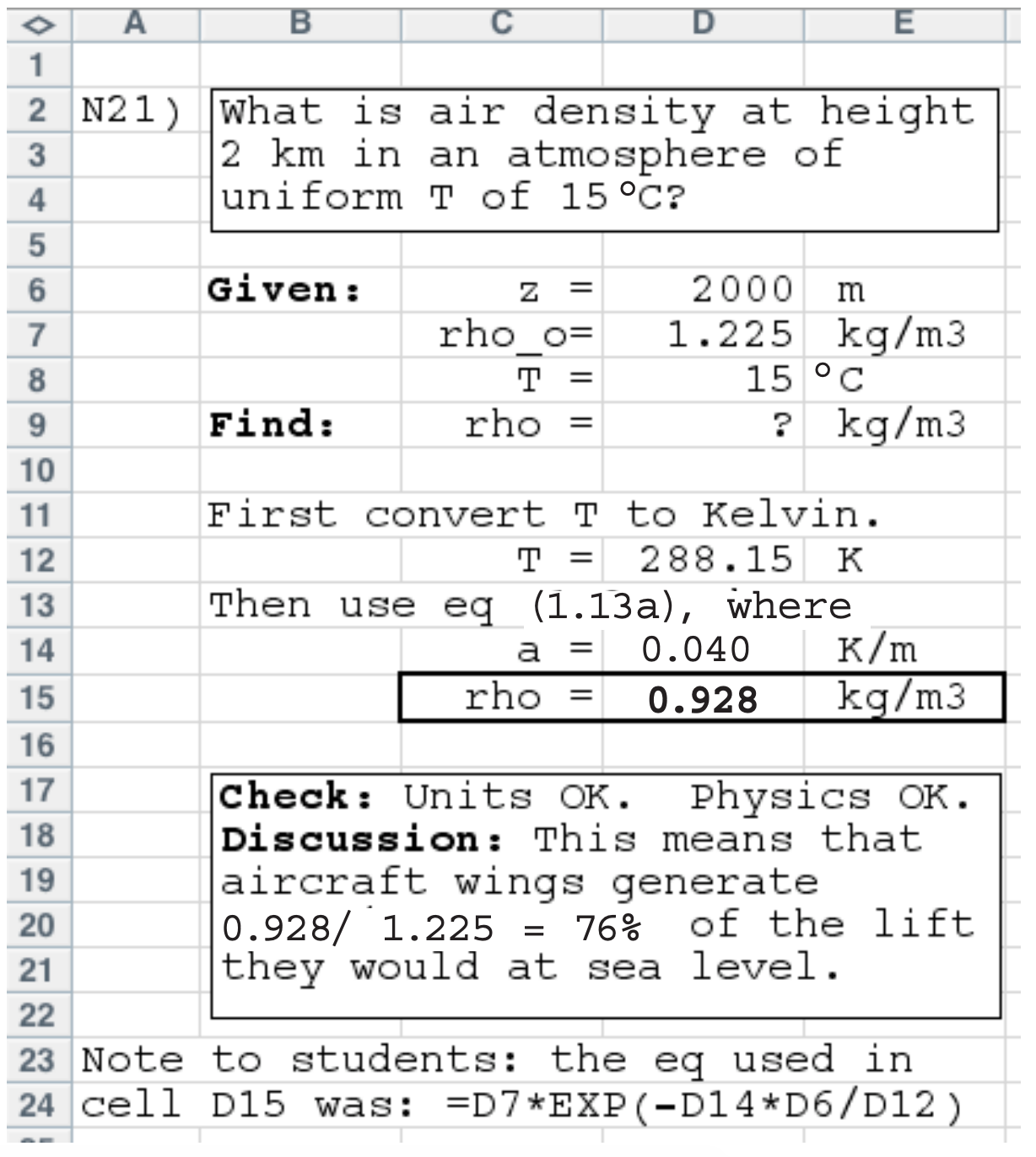
Finally, most of the exercises have multiple parts to them. Your instructor need assign only one of the parts for you to gain the skills associated with that exercise. Many of the numerical problems are similar to Sample Applications presented earlier in the chapter. Thus, you can try to do the Sample Application first, and if you get the same answer as I did, then you can be more confident in getting the right answer when you re-solve the exercise part assigned by your instructor. Such re-solutions are trivial if you use a computer spreadsheet (Figure 1.13) or other similar program to solve the numerical exercises.

Format Guidelines for Your Homework
Good scientists and engineers are not only creative, they are methodical, meticulous, and accurate. To encourage you to develop these good habits, many instructors require your homework to be written in a clear, concise, organized, and consistent format. Such a format is described below, and is illustrated in all the Sample Applications in this book. The format below closely follows steps you typically take in problem solving (Appendix A).
Format:
- Give the exercise number, & restate the problem.
- Start the solution section by listing the “Given” known variables (WITH THEIR UNITS).
- List the unknown variables to find, with units.
- Draw a sketch if it clarifies the scenario.
- List the equation(s) you will use.
- Show all your intermediate steps and calculations (to maximize your partial credit), and be sure to ALWAYS INCLUDE UNITS with the numbers when you plug them into eqs.
- Put a box around your final answer, or underline it, so the grader can find it on your page amongst all the coffee and pizza stains.
- Always check the value & units of your answer.
- Briefly discuss the significance of the answer.
Example:
Problem: What is air density at height 2 km in an isothermal atmosphere of temperature 15°C?
Find the Answer
Given: z = 2000 m
ρo = 1.225 kg m–3
T = 15°C = 288.15 K
Find: ρ = ? kg m–3
Use eq. (1.13a): ρ = (1.225 kg m–3)· exp[(–0.040K m–1)·(2000m)/288K]
ρ = 0.928 kg m–3
Check: Units OK. Physics reasonable.
Exposition: (ρo – ρ)/ρo ≈ 0.24. This means that aircraft wings generate 24% less lift, aircraft engines generate 24% less power, and propellers 24% less thrust because of the reduced air density. This compounding effect causes aircraft performance to decrease rapidly with increasing altitude, until the ceiling is reached where the plane can’t climb any higher.
Figure 1.13 shows the solution of this problem on a computer spreadsheet.


