16.6: A Tropical Cyclone Model

Although tropical cyclones are quite complex and not fully understood, we can build an idealized model that mimics some of the real features.

16.6.1. Pressure Distribution

Eye pressures of 95 to 99 kPa at sea level are common in tropical cyclones, although a pressure as low as P_eye = 87 kPa has been measured. One measure of tropical cyclone strength is the pressure difference ∆P_max between the eye and the surrounding ambient environment where P_∞ = 101.3 kPa:

\(\ \begin{align} \Delta P_{\max }=P_{\infty}-P_{e y e}\tag{16.10}\end{align}\)

The surface pressure distribution across a tropical cyclone can be approximated by:

\(\ \begin{align} \frac{\Delta P}{\Delta P_{\max }}=\left\{\begin{array}{ll}\frac{1}{5} \cdot\left(\frac{R}{R_{0}}\right)^{4} & \text { for } R \leq R_{0} \\ \left[1-\frac{4}{5} \cdot \frac{R_{0}}{R}\right] & \text { for } R>R_{0}\end{array}\right.\tag{16.11}\end{align}\)

where ∆P = P(R) – P_eye , and R is the radial distance from the center of the eye. This pressure distribution is plotted in Fig 16.31, with data points from two tropical cyclones.

Figure 16.31 Surface pressure distribution across a tropical cyclone. Model is eq. (16.11).

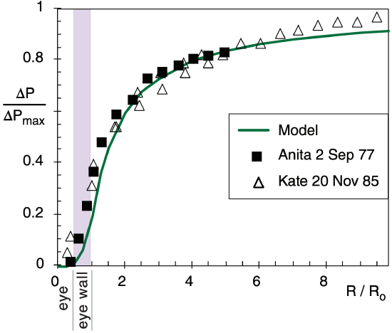
R_o is the critical radius where the maximum tangential winds are found. In the tropical cyclone model presented here, R_o is twice the radius of the eye. Eyes range from 4 to 100 km in radius, with average values of 15 to 30 km. Thus, one anticipates average values of critical radius of 30 < R_o < 60 km, with an observed range of 8 < R_o < 200 km.

16.6.2. Tangential Velocity

To be classified as a tropical cyclone, the sustained winds (averaged over 1-minute) must be 33 m s^–1 or greater near the surface. While most anemometers are unreliable at extreme wind speeds, maximum tropical cyclone winds have been reported in the 75 to 95 m s^–1 range.

Figure 16.32 Maximum sustained winds around a tropical cyclone increase as sea-level pressure in the eye decreases.

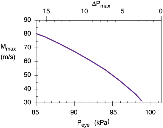
As sea-level pressure in the eye decreases, maximum tangential surface winds M_max around the eye wall increase (Fig. 16.32). An empirical approximation for this relationship, based on Bernoulli’s equation (see the Regional Winds chapter), is :

\(\ \begin{align} M_{\max }=a \cdot\left(\Delta P_{\max }\right)^{1 / 2}\tag{16.12}\end{align}\)

where a = 20 (m s^–1)·kPa^–1/2 .

Sample Application

What max winds are expected if the tropical cyclone eye has surface pressure of 95 kPa?

Find the Answer

Given: P_{B eye} = 95 kPa, Assume P_{B ∞} = 101.3 kPa

Find: M_max = ? m s^–1.

Assume translation speed can be neglected.

Use eq. (16.12):

M_max = [20 (m s^–1)·kPa^–1/2]·(101.3–95kPa)^1/2 = 50 m s^–1

Check: Units OK. Physics OK.

Exposition: This is a category 3 tropical cyclone on the Saffir-Simpson tropical cyclone Wind Scale.

If winds are assumed to be cyclostrophic (not the best assumption, because drag against the sea surface and Coriolis force are neglected), then the previous approximation for pressure distribution (eq. 16.11) can be used to give a distribution of tangential velocity M_tan (relative to the eye) in the boundary layer:

\(\ \begin{align} \frac{M_{\tan }}{M_{\max }}=\left\{\begin{array}{ll}\left(R / R_{0}\right)^{2} & \text { for } R \leq R_{0} \\ \left(R_{0} / R\right)^{1 / 2} & \text { for } R>R_{0}\end{array}\right.\tag{16.13}\end{align}\)

where the maximum velocity occurs at critical radius R_o (assumed to be twice the radius of the eye). This is plotted in Fig. 16.33, with data points from a few tropical cyclones.

Figure 16.33 Tangential winds near the surface at various radii around tropical cyclones. Model is eq. (16.13).

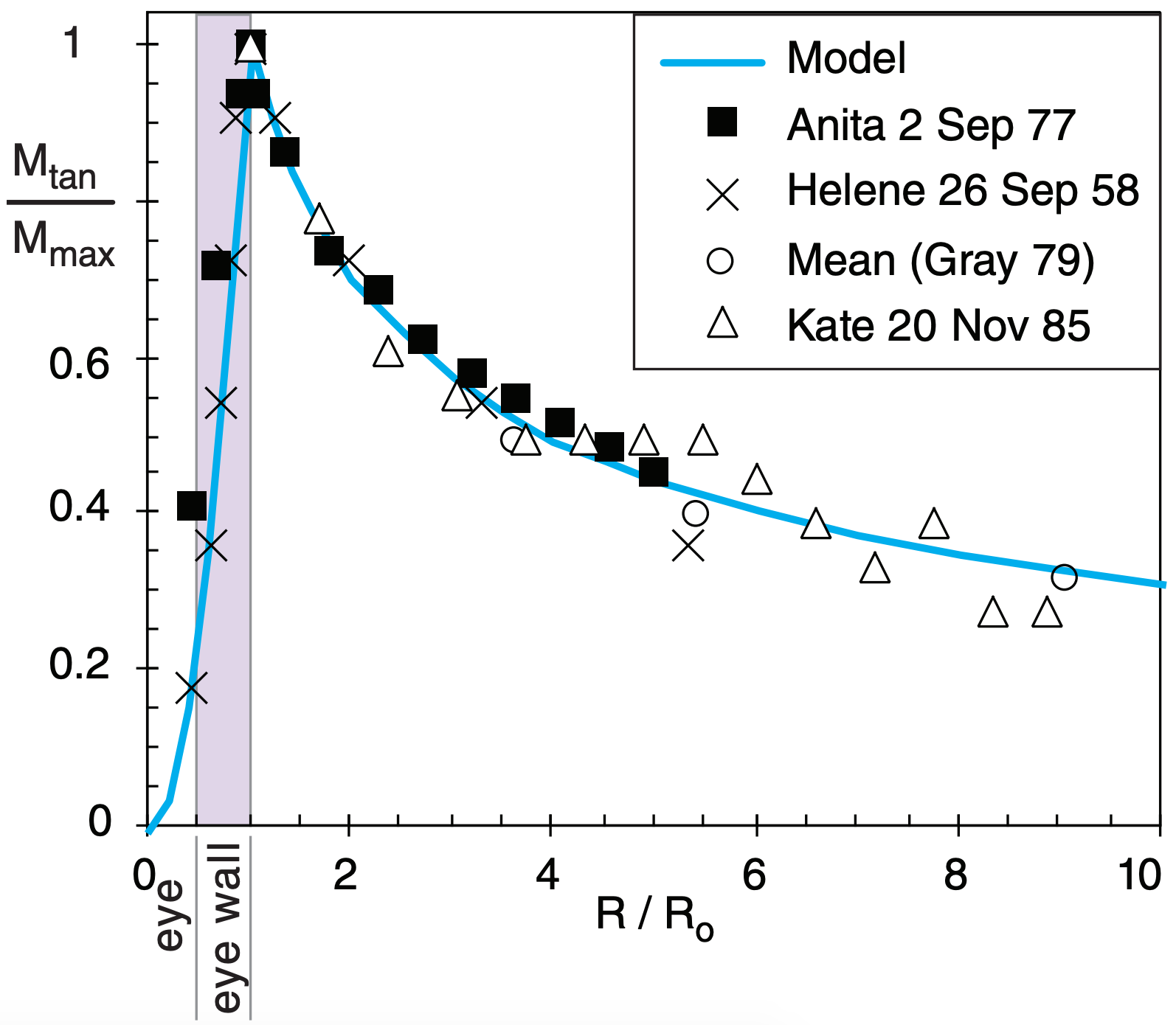
For the tropical cyclones plotted in Fig. 16.33, the critical radius of maximum velocity was in the range of R_o = 20 to 30 km. This is a rough definition of the outside edge of the eye wall for these tropical cyclones, within which the heaviest precipitation falls. The maximum velocity for these storms was M_max = 45 to 65 m s^–1.

Winds in Fig. 16.33 are relative to those in the eye. However, the whole tropical cyclone including the eye is often moving. Tropical cyclone translation speeds (movement of the center of the storm) can be as slow as M_t = 0 to 5 m s^–1 as they drift westward in the tropics, and as fast as 25 m s^–1 as they later move poleward. Average translation speeds of tropical cyclones over the ocean are M_t = 10 to 15 m s^–1.

Figure 16.34 Max 1-minute total sustained surface winds (m s^–1) around Hurricane Isabel, 0730 UTC 18 Sep 2003. M_{max total} = 42 m s^–1, and P_eye ≈ 95.7 kPa. Arrow shows translation toward 325° at 5.5 m s^–1. The Saffir-Simpson Hurricane Wind Scale is based on the fastest total sustained wind (rotational + translational) found anywhere in the hurricane.

Figure 16.35 Sum of the modeled tangential winds relative to the eye and the translation speed (10 m s^–1) of the eye, for a hypothetical tropical cyclone. Assumes M_max = 50 m s^–1 relative to the eye, Ro = 25 km, and uses a coordinate system with the x-axis aligned in the same direction as the translation vector. Purple shading indicates the eye wall locations.

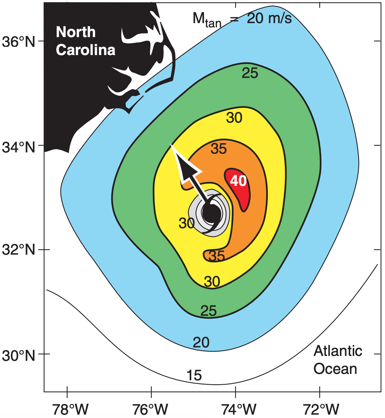
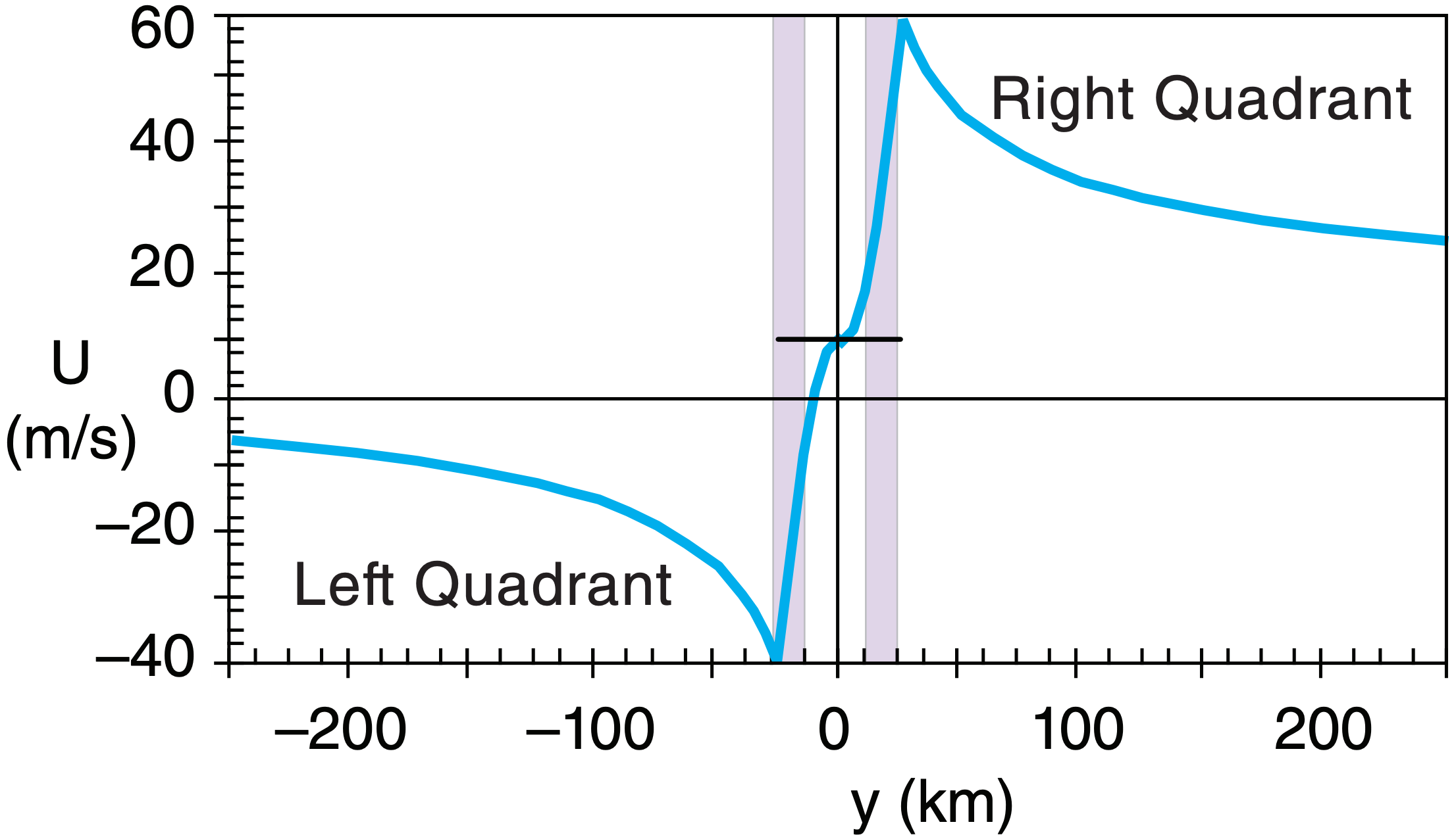
The total wind speed relative to the surface is the vector sum of the translation speed and the rotation speed. On the right quadrant of the storm relative to its direction of movement in the Northern Hemisphere, the translation speed adds to the rotation speed. Thus, tropical cyclone winds are fastest in the tropical cyclone’s right quadrant (Fig. 16.34). On the left the translation speed subtracts from the tangential speed, so the fastest total speed in the left quadrant is not as strong as in the right quadrant (Fig. 16.35).

Total speed relative to the surface determines ocean wave and surge generation. Thus, the right quadrant of the storm near the eye wall is most dangerous. Also, tornadoes are likely there.

16.6.3. Radial Velocity

For an idealized tropical cyclone, boundary-layer air is trapped below the top of the boundary layer as winds converge horizontally toward the eye wall. Horizontal continuity in cylindrical coordinates requires:

\(\ \begin{align} M_{r a d} \cdot R= constant \tag{16.14}\end{align}\)

where M_rad is the radial velocity component, which is negative for inflow. Thus, starting from far outside the tropical cyclone, as R decreases toward R_o, the magnitude of inflow must increase. Inside of R_o, thunderstorm convection removes air mass vertically, implying that horizontal continuity is no longer satisfied.

As distance from the eyewall decreases, surface winds increase, which cause increasing wave height and ocean-surface roughness. The resulting turbulent drag against the ocean surface tends to couple the radial and tangential velocities, which we can approximate by M_rad ∝ M_tan² . Drag-induced inflow such as this eventually converges and forces ascent via the boundary-layer pumping process (see the Atmospheric Forces & Winds chapter).

The following equations utilize the concepts above, and are consistent with the tangential velocity in the previous subsection:

\(\ \begin{align} \frac{M_{r a d}}{M_{\max }}=\left\{\begin{array}{l}-\frac{R}{R_{0}} \cdot\left[\frac{1}{5}\left(\frac{R}{R_{0}}\right)^{3}+\frac{1}{2} \frac{W_{s}}{M_{\max }} \frac{R_{0}}{z_{i}}\right] \text { for } R \leq R_{0} \\ -\frac{R_{0}}{R} \cdot\left[\frac{1}{5}+\frac{1}{2} \cdot \frac{W_{s}}{M_{\max }} \cdot \frac{R_{o}}{z_{i}}\right] \quad \text { for } R>R_{0}\end{array}\right.\tag{16.15}\end{align}\)

where W_s is negative, and represents the average subsidence velocity in the eye. Namely, the horizontal area of the eye, times W_s, gives the total kinematic mass flow downward in the eye. The boundary-layer depth is z_i , and M_max is still the maximum tangential velocity.

Figure 16.36 Radial winds in a tropical cyclone boundary layer. (Negative values indicate inward motion, converging toward R/R_o = 0.)

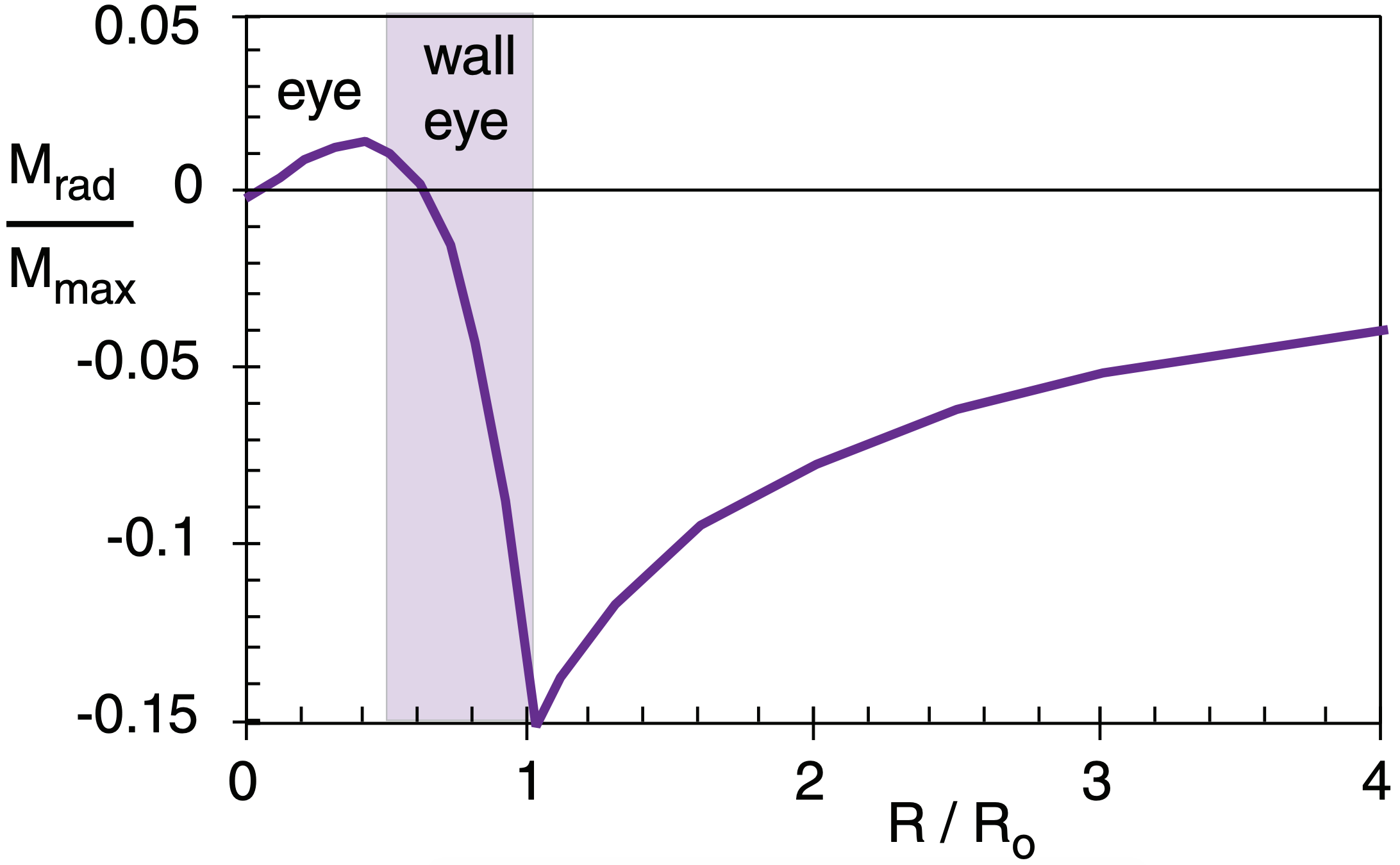
For example, Fig. 16.36 shows a plot of the equations above, using z_i = 1 km, R_o = 25 km, M_max = 50 m s^–1, and W_s = –0.2 m s^–1. In the eye, subsidence causes air to weakly diverge (positive M_rad) toward the eye wall. Inside the eye wall, the radial velocity rapidly changes to inflow (negative M_rad), reaching an extreme value of –7.5 m s^–1 for this case. Outside of the eye wall, the radial velocity smoothly decreases as required by horizontal mass continuity.

16.6.4. Vertical Velocity

At radii less than R_o, the converging air rapidly piles up, and rises out of the boundary layer as thunderstorm convection within the eye wall. The vertical velocity out of the top of the boundary layer, as found from mass continuity, is

\(\ \begin{align} \frac{W}{M_{\max }}=\left\{\begin{array}{ll}\left[\frac{z_{i}}{R_{o}}\left(\frac{R}{R_{o}}\right)^{3}+\frac{W_{s}}{M_{\max }}\right] & \text { for } R<R_{o} \\ 0 & \text { for } R>R_{o}\end{array}\right.\tag{16.16}\end{align}\)

For simplicity, we are neglecting the upward motion that occurs in the spiral rain bands at R > R_o.

As before, W_s is negative for subsidence. Although subsidence acts only inside the eye for real tropical cyclones, the relationship above applies it every where inside of R_o for simplicity. Within the eye wall, the upward motion overpowers the subsidence, so our simplification is of little consequence.

Figure 16.37 Vertical velocity at various radii around tropical cyclones, out of the top of the boundary layer. W_s = –0.2 m s^–1 in the eye.

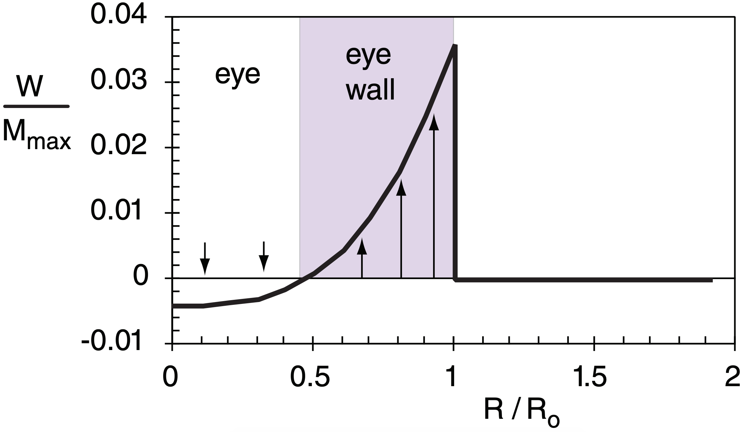
Using the same values as for the previous figure, the vertical velocity is plotted in Fig. 16.37. The maximum upward velocity is 1.8 m s^–1 in this case, which represents an average around the eye wall. Updrafts in individual thunderstorms can be much faster.

Subsidence in the eye is driven by the non-hydrostatic part of the pressure perturbation (Fig. 16.29). Namely, the pressure gradient (shown by the dashed green line between X’s in that Fig.) that pushes air upward is weaker than gravity pulling down. This net imbalance forces air downward in the eye.

16.6.5. Temperature

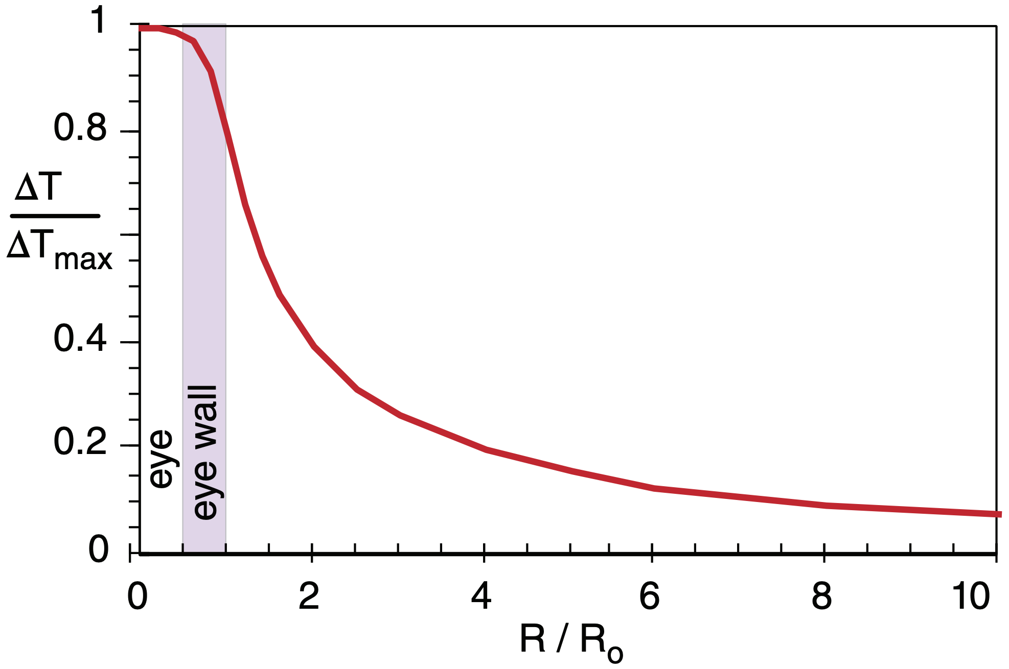
Suppose that the pressure difference between the eye and surroundings at the top of the tropical cyclone is equal and opposite to that at the bottom. From eq. (16.5) the temperature T averaged over the tropical cyclone depth at any radius R is found from:

\(\ \begin{align} \Delta T(R)=c \cdot\left[\Delta P_{\max }-\Delta P(R)\right]\tag{16.17}\end{align}\)

where c = 1.64 K kPa^–1, the pressure difference at the bottom is ∆P = P(R) – P_eye, and the temperature difference averaged over the whole tropical cyclone depth is ∆T(R) = T_eye – T(R). When used with eq. (16.11), the result is:

\(\ \begin{align} \frac{\Delta T}{\Delta T_{\max }}=\left\{\begin{array}{ll}1-\frac{1}{5} \cdot\left(\frac{R}{R_{0}}\right)^{4} & \text { for } R \leq R_{0} \\ \frac{4}{5} \cdot \frac{R_{0}}{R} & \text { for } R>R_{0}\end{array}\right.\tag{16.18}\end{align}\)

where ∆T_max = T_eye – T_∞ = c · ∆P_max , and c = 1.64 K kPa–1. This is plotted in Fig. 16.38.

Figure 16.38 Temperature distribution, averaged over a 15 km-thick tropical cyclone, showing the warm core.

16.6.6. Composite Picture

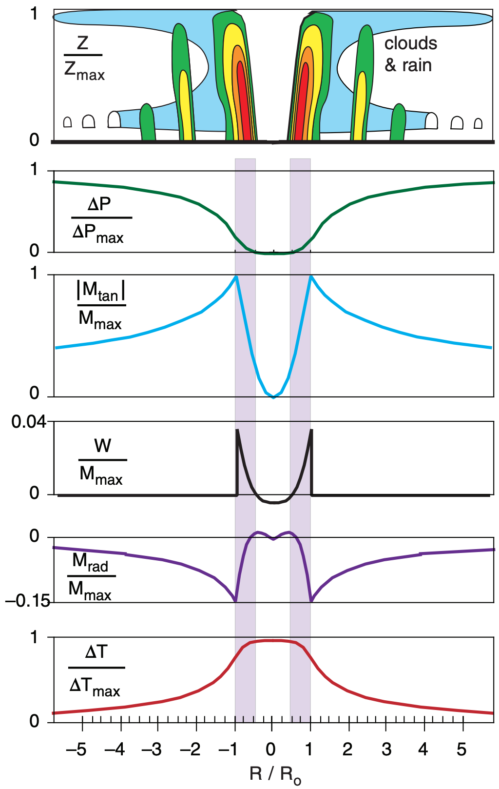
A coherent picture of tropical cyclone structure can be presented by combining all of the idealized models described above. The result is sketched in Fig. 16.39. For real tropical cyclones, sharp cusps in the velocity distribution would not occur because of vigorous turbulent mixing in the regions of strong shear.

Figure 16.39 Composite tropical cyclone structure based on the idealized model. Pressure differences are at sea level. All horizontal velocities are in the boundary layer, while vertical velocity is across the top of the boundary layer. Temperature differences are averaged over the whole tropical cyclone depth. Purple vertical bands indicate eyewall locations.

Sample Application

A tropical cyclone of critical radius R_o = 25 km has a central pressure of 90 kPa. Find the wind components, vertically-averaged temperature excess, and pressure at radius 40 km from the center. Assume W_s = –0.2 m s^–1 in the eye, and z_i = 1 km.

Find the Answer

Given: P_{B eye} = 90 kPa, R_o = 25 km, R = 40 km, W_s = –0.2 m s^–1, and z_i = 1 km.

Find: P = ? kPa, T = ? °C, M_tan = ? m s^–1, M_rad = ? m s^–1, W = ? m s^–1

Assume P_{B ∞} = 101.3 kPa

Figure: Similar to Fig. 16.39. Note that R > R_o.

First, find maximum values:

∆P_max = (101.3 – 90kPa) = 11.3 kPa

Use eq. (16.12):

M_max = [(20m s^–1)·kPa^–1/2]·(11.3kPa)^1/2 = 67 m s^–1

∆T_max = c·∆P_max=(1.64 K kPa^–1)·(11.3kPa) = 18.5°C

Use eq. (16.11):

\(\Delta P=(11.3 \mathrm{kPa}) \cdot\left[1-\frac{4}{5} \cdot \frac{25 \mathrm{km}}{40 \mathrm{km}}\right]=5.65 \mathrm{kPa}\)

P = P_eye + ∆P = 90 kPa + 5.65 kPa = 95.65 kPa.

Use eq. (16.18):

\(\Delta T=\left(18.5^{\circ} \mathrm{C}\right) \cdot \frac{4}{5} \cdot \frac{(25 \mathrm{km})}{(40 \mathrm{km})}=\underline{\mathbf{9.25^{\circ} \mathrm{C}}}\)

averaged over the whole tropical cyclone depth.

Use eq. (16.13):

\(M_{\tan }=(67 \mathrm{m} / \mathrm{s}) \cdot \sqrt{\frac{25 \mathrm{km}}{40 \mathrm{km}}}=\underline{\mathbf{53 \mathrm{m} \mathrm{s}^{-1}}}\)

Use eq. (16.15):

\(M_{r a d}=-(67 \mathrm{m} / \mathrm{s}) \cdot \frac{(25 \mathrm{km})}{(40 \mathrm{km})} \cdot\left[\frac{1}{5}+\frac{1}{2} \cdot \frac{(-0.2 \mathrm{m} / \mathrm{s})}{(67 \mathrm{m} / \mathrm{s})} \cdot \frac{(25 \mathrm{km})}{(1 \mathrm{km})}\right]\)

M_rad = –6.8 m s^–1

Use eq. (16.16): W = 0 m s^–1

Check: Units OK. Physics OK.

Exposition: Using P_eye in Table 16-7, the approximate Saffir-Simpson category of this tropical cyclone is borderline between levels 4 and 5, and thus is very intense.