12.4: Geostrophic Adjustment - Part 3

12.4.1. Winds in the Cold Air

Why does cold dense air from the poles not spread out over more of the Earth, like a puddle of water? Coriolis force is the culprit, as shown next.

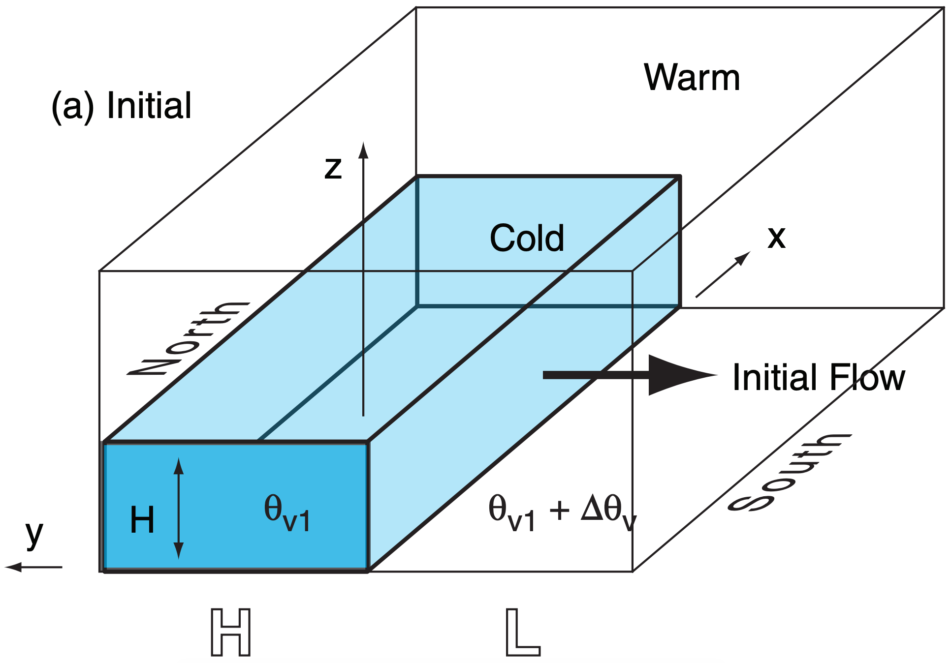
Picture two air masses initially adjacent (Fig. 12.17a). The cold airmass has initial depth H and uniform virtual potential temperature θ_v1. The warm airmass has uniform virtual potential temperature θ_v1 + ∆θ_v. The average absolute virtual temperature is \(\ \overline{T_v} \). In the absence of rotation of the coordinate system, you would expect the cold air to spread out completely under the warm air due to buoyancy, reaching a final state that is horizontally homogeneous.

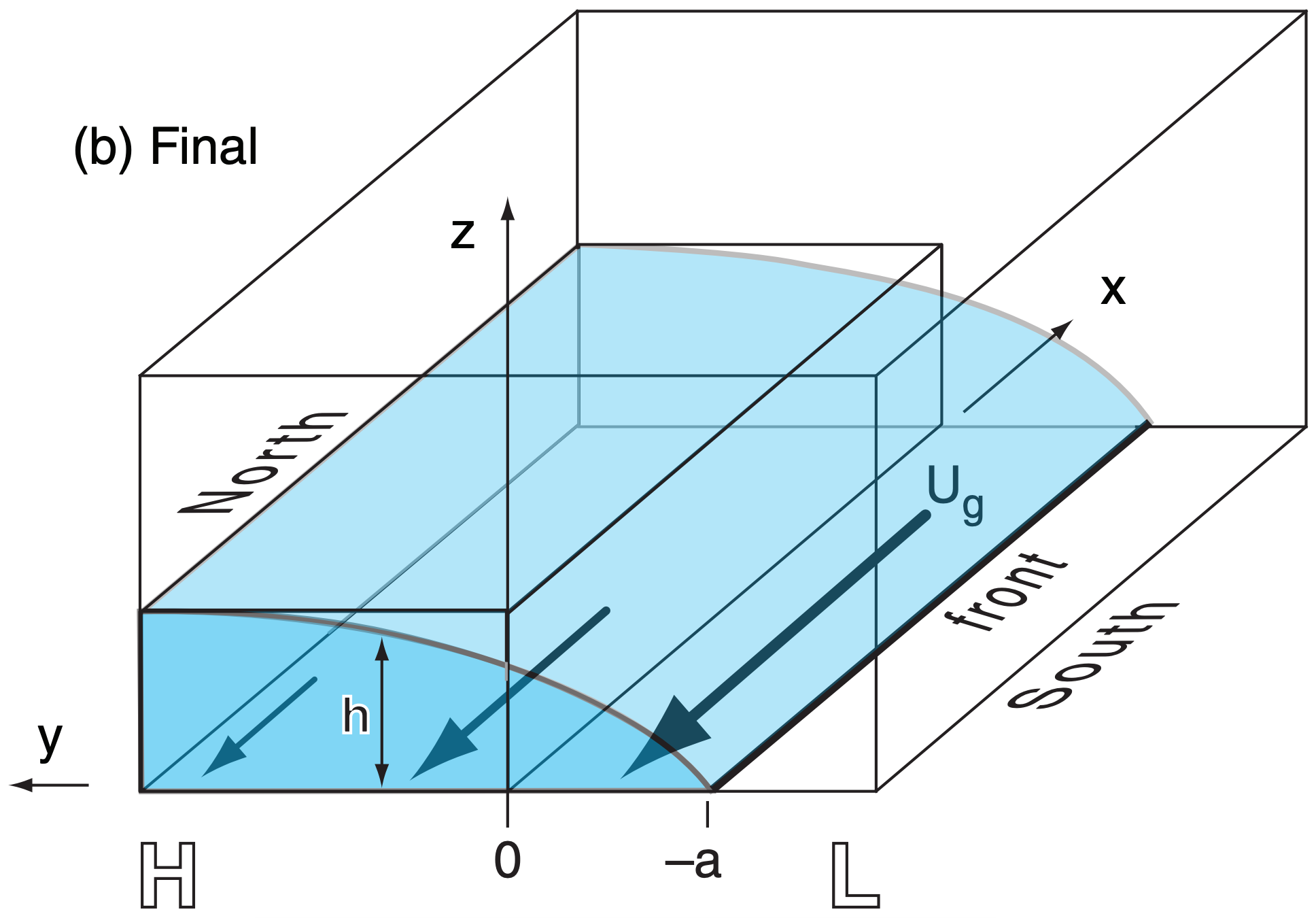
However, on a rotating Earth, the cold air experiences Coriolis force (to the right in the Northern Hemisphere) as it begins to move southward. Instead of flowing across the whole surface, the cold air spills only distance a before the winds have turned 90°, at which point further spreading stops (Fig. 12.17b).

At this quasi-equilibrium, pressure-gradient force associated with the sloping cold-air interface balances Coriolis force, and there is a steady geostrophic wind U_g from east to west. The process of approaching this equilibrium is called geostrophic adjustment, as was discussed in the previous chapter. Real atmospheres never quite reach this equilibrium.

At equilibrium, the final spillage distance a of the front from its starting location equals the external Rossby-radius of deformation, λ_R:

\(\ \begin{align} a=\lambda_{R}=\frac{\sqrt{|g| \cdot H \cdot \Delta \theta_{v} / \overline{T_{v}}}}{f_{c}}\tag{12.5}\end{align}\)

where f_c is the Coriolis parameter and |g| = 9.8 m s^–2 is gravitational acceleration magnitude.

The geostrophic wind U_g in the cold air at the surface is greatest at the front (neglecting friction), and exponentially decreases behind the front:

\(\ \begin{align} U_{g}=-\sqrt{|g| \cdot H \cdot\left(\Delta \theta_{v} / \overline{T_{v}}\right)} \cdot \exp \left(-\frac{y+a}{a}\right)\tag{12.6}\end{align}\)

for –a ≤ y ≤ ∞ . The depth of the cold air h is:

\(\ \begin{align} h=H \cdot\left[1-\exp \left(-\frac{y+a}{a}\right)\right]\tag{12.7}\end{align}\)

which smoothly increases to depth H well behind the front (at large y).

Figs. 12.17 are highly idealized, having airmasses of distinctly different temperatures with a sharp interface in between. For a fluid with a smooth continuous temperature gradient, geostrophic adjustment occurs in a similar fashion, with a final equilibrium state as sketched in Fig. 12.18. The top of this diagram represents the top of the troposphere, and the top wind vector represents the jet stream.

Figure 12.17 Geostrophic adjustment of a cold front. (a) Initial state. (b) Final state is in dynamic equilibrium, which is never quite attained in the real atmosphere. Cold air is shaded light blue.

Figure 12.18 Final dynamic state after geostrophic adjustment within an environment containing continuous temperature gradients. Arrows represent geostrophic wind. Shaded areas are isobaric surfaces. H and L indicate high and low pressures relative to surrounding pressures at the same altitude. Dot-circle represents the tip of an arrow pointing toward the reader, x-circle represents the tail feathers of an arrow pointing into the page.

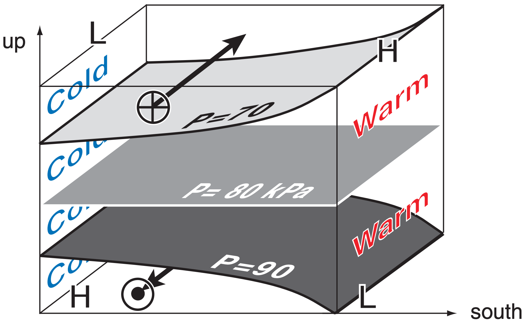
This state has high surface pressure under the cold air, and low surface pressure under the warm air (see the General Circulation chapter). On the cold side, isobaric surfaces are more-closely spaced in height than on the warm side, due to the hypsometric relationship. This results in a pressure reversal aloft, with low pressure (or low heights) above the cold air and high pressure (or high heights) above the warm air.

Horizontal pressure gradients at low and high altitudes create opposite geostrophic winds, as indicated in Fig. 12.18. Due to Coriolis force, the air represented in Fig. 12.18 is in equilibrium; namely, the cold air does not spread any further.

This behavior of the cold airmass is extremely significant. It means that the planetary-scale flow, which is in approximate geostrophic balance, is unable to complete the job of redistributing the cold air from the poles and warm air from the tropics. Yet some other process must be acting to complete the job of redistributing heat to satisfy the global energy budget (in the General Circulation chapter).

That other process is the action of cyclones and Rossby waves. Many small-scale, short-lived cyclones are not in geostrophic balance, and they can act to move the cold air further south, and the warm air further north. These cyclones feed off the potential energy remaining in the large-scale flow, namely, the energy associated with horizontal temperature gradients. Such gradients have potential energy that can be released when the colder air slides under the warmer air (see Fig. 11.1).

HIGHER MATH • Geostrophic Adjustment

We can verify that the near-surface (frictionless) geostrophic wind is consistent with the sloping depth of cold air. The geostrophic wind is related to the horizontal pressure gradient at the surface by:

\(\ \begin{align} U_{g}=-\frac{1}{\rho \cdot f_{c}} \cdot \frac{\Delta P}{\Delta y}\tag{10.26a}\end{align}\)

Assume that the pressure at the top of the cold airmass in Figs. 12.17 equals the pressure at the same altitude h in the warm airmass. Thus, surface pressures will be different due to only the difference in weight of air below that height.

Going from the top of the sloping cold airmass to the bottom, the vertical increase of pressure is given by the hydrostatic eq: ∆P_cold = −ρ_cold · |g| · h

A similar equation can be written for the warm air below h. Thus, at the surface, the difference in pressures under the cold and warm air masses is:

∆P = - |g| · h · (ρ_cold - ρ_warm )

multiplying the RHS by \(\bar{\rho} / \bar{\rho}\), where \(\bar{\rho}\) is an average density, yields:

\(\Delta P=-|g| \cdot h \cdot \bar{\rho} \cdot\left[\left(\rho_{c o l d}-\rho_{w a r m}\right) / \bar{\rho}\right]\)

As was shown in the Buoyancy section of the Stability chapter, use the ideal gas law to convert from density to virtual temperature, remembering to change the sign because the warmer air is less dense. Also, ∆T_v =∆θ_v. Thus: \(\Delta P=-|g| \cdot h \cdot \bar{\rho} \cdot\left[\left(\theta_{v \text { warm }}-\theta_{v \text { cold }}\right) / \bar{T}_{v}\right]\)

where this is the pressure change in the negative y direction.

Plugging this into eq. (10.26a) gives:

\(U_{g}=-\frac{|g| \cdot\left(\Delta \theta_{v} / T_{v}\right)}{f_{c}} \cdot \frac{\Delta h}{\Delta y}\)

which we can write in differential form:

\(\ \begin{align} u_{g}=-\frac{|g| \cdot\left(\Delta \theta_{v} / T_{v}\right)}{f_{c}} \cdot \frac{\partial h}{\partial y}\tag{b}\end{align}\)

The equilibrium value of h was given by eq. (12.7):

\(\ \begin{align} h=H \cdot\left[1-\exp \left(-\frac{y+a}{a}\right)\right]\tag{12.7}\end{align}\)

Thus, the derivative is:

\(\frac{\partial h}{\partial y}=\frac{H}{a} \cdot \exp \left(-\frac{y+a}{a}\right)\)

Plugging this into eq. (b) gives:

\(\ \begin{align} U_{g}=-\frac{|g| \cdot\left(\Delta \theta_{v} / T_{v}\right)}{f_{c}} \cdot \frac{H}{a} \cdot \exp \left(-\frac{y+a}{a}\right)\tag{c}\end{align}\)

But from eq. (12.5) we see that:

\(\ \begin{align} f_{c} \cdot a=f_{c} \cdot \lambda_{R}=\sqrt{|g| \cdot H \cdot\left(\Delta \theta_{v} / T_{v}\right)}\tag{12.5}\end{align}\)

Eq. (c) then becomes:

\(\ \begin{align} U_{g}=-\sqrt{|g| \cdot H \cdot\left(\Delta \theta_{v} / T_{v}\right)} \cdot \exp \left(-\frac{y+a}{a}\right)\tag{12.6}\end{align}\)

Thus, the wind is consistent (i.e., geostrophically balanced) with the sloping height.

Sample Application

A cold airmass of depth 1 km and virtual potential temperature 0°C is embedded in warm air of virtual potential temperature 20°C. Find the Rossby deformation radius, the maximum geostrophic wind speed, and the equilibrium depth of the cold airmass at y = 0. Assume f_c = 10^–4 s^–1 .

Find the Answer

Given: \(\ \overline{T_v}\) = 280 K, ∆θ_v = 20 K, H = 1 km, f_c = 10^–4 s^–1 .

Find: a = ? km, U_g = ? m s^–1 at y = –a, and h = ? km at y = 0.

Use eq. (12.5):

\(a=\frac{\sqrt{\left(9.8 \mathrm{m} \cdot \mathrm{s}^{-2}\right) \cdot(1000 \mathrm{m}) \cdot(20 \mathrm{K}) /(280 \mathrm{K})}}{10^{-4} \mathrm{s}^{-1}}\)

= 265 km

Use eq. (12.6):

\(U_{g}=-\sqrt{\left(9.8 \mathrm{m} \cdot \mathrm{s}^{-2}\right)(1000 \mathrm{m})(20 \mathrm{K}) /(280 \mathrm{K})} \cdot \exp (0)\)

= –26.5 m s^–1

Use eq. (12.7):

\(h=(1 \mathrm{km}) \cdot[1-\exp (-1)]\) = 0.63 km

Check: Units OK. Physics OK.

Exposition: Frontal-zone widths on the order of a = 200 km are small compared to lengths (1000s km).

12.4.2. Winds in the Warm Over-riding Air

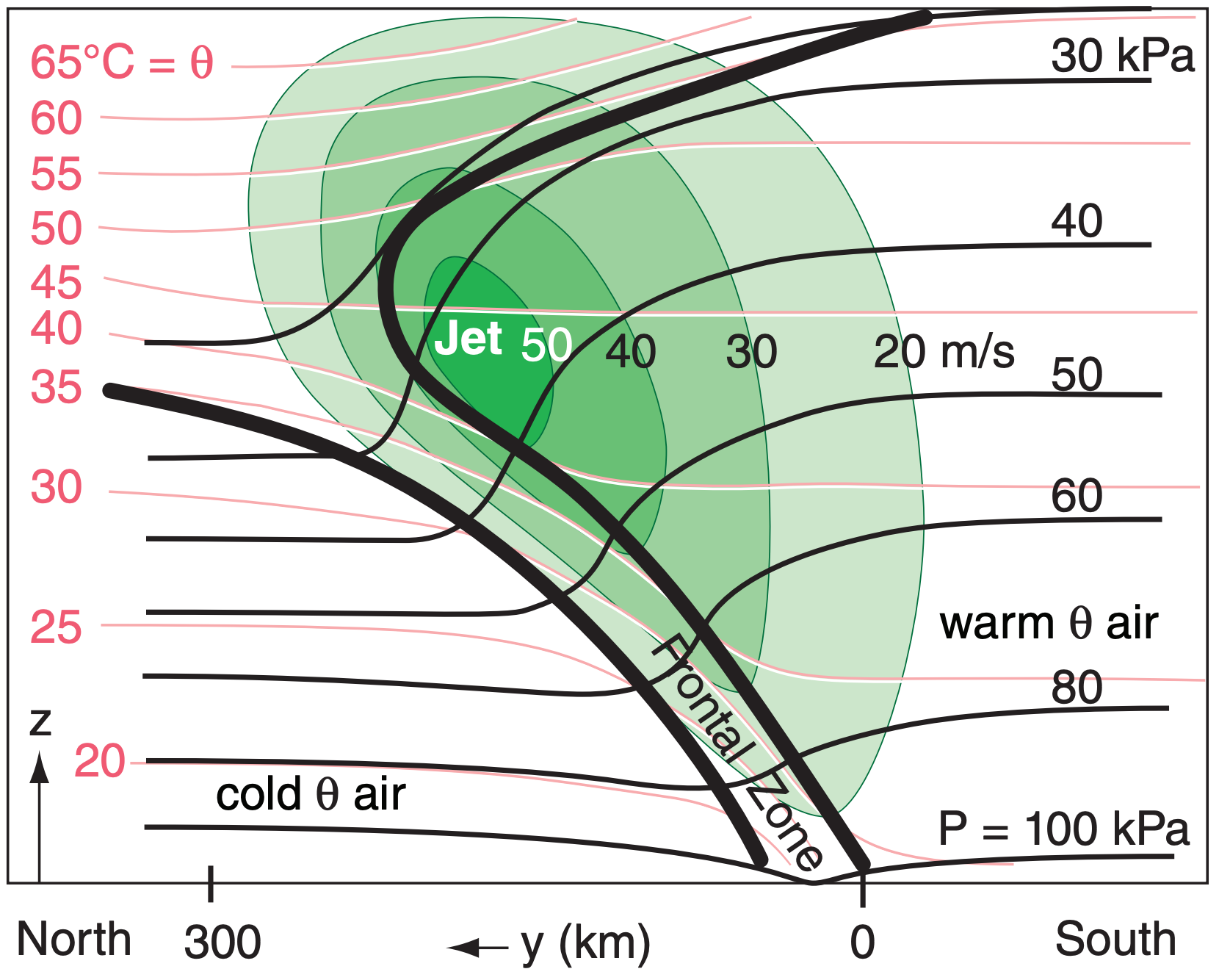
Across the frontal zone is a stronger-than-background horizontal temperature gradient. In many fronts, the horizontal temperature gradient is strongest near the surface, and weakens with increasing altitude.

The thermal-wind relationship tells us that the geostrophic wind will increase with height in strong horizontal temperature gradients. If the frontal zone extends vertically over a large portion of the troposphere, then the wind speed will continue to increase with height, reaching a maximum near the tropopause.

Thus, jet streams are associated with frontal zones. The jet blows parallel to the frontal zone, with greatest wind speeds on the warm side of the frontal zone. If the cold air is advancing as a cold front, then this jet is known as a pre-frontal jet.

This is illustrated in Fig. 12.19. Plotted are isentropes, isobars, isotachs, and the frontal zone. The cross-frontal direction is north-south in this figure, causing a pre-frontal jet from the West (blowing into the page, in this diagram).

Figure 12.19 Vertical section across a cold front in the N. Hemisphere. Thick lines outline the frontal zone in the troposphere, and show the tropopause in the top of the graph. Medium black lines are isobars. Thin pink lines are isentropes. Green shaded areas indicate isotachs, for a jet that blows from the West (into the page).

12.4.3. Frontal Vorticity

Combining the cold-air-side winds from Fig. 12.17b and warm-air-side winds from Fig. 12.19 into a single diagram yields Fig. 12.20. In this sketch, the warm air aloft and south of the front has geostrophic winds from the west, while the cold air near the ground has geostrophic winds from the east.

Figure 12.20 Sketch of cold front, combining winds (thick straight grey arrow) in the cold air (light blue shading) from Fig. 12.17b with the winds in the warm air (thick white arrow) from Fig. 12.19. These winds cause shear across the front, shown with the black arrows. This shear is associated with positive (cyclonic) relative vorticity of the geostrophic wind (thin curved grey arrows).

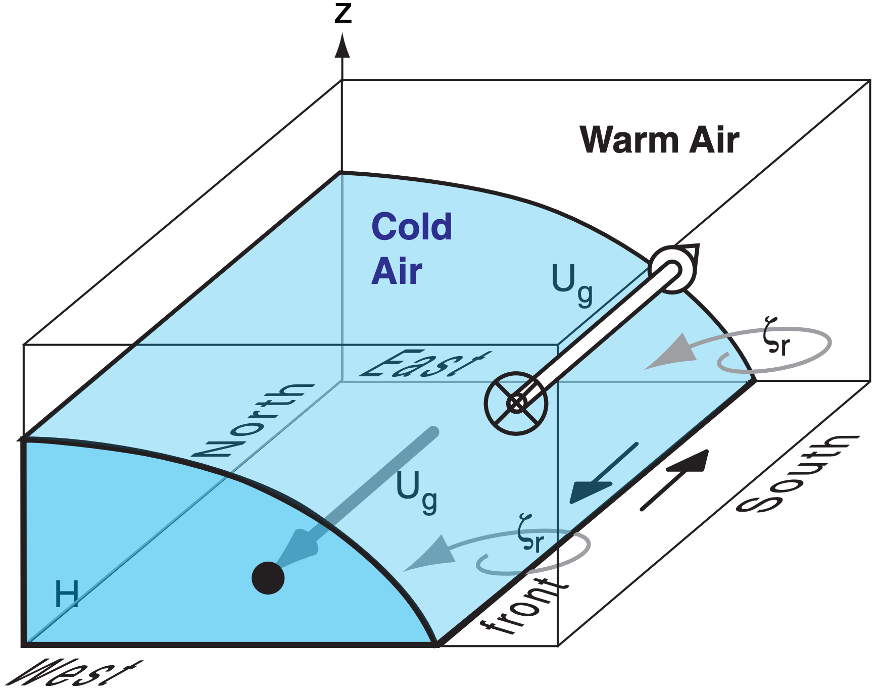
Thus, across the front, ∆U_g/∆y is negative, which means that the relative vorticity (eq. 11.20) of the geostrophic wind is positive (ζ_r = +) at the front (grey curved arrows in Fig. 12.20). In fact, cyclonic vorticity is found along fronts of any orientation. Also, stronger density contrasts across fronts cause greater positive vorticity.

Also, frontogenesis (strengthening of a front) is often associated with horizontal convergence of air from opposite sides of the front (see next section). Horizontal convergence implies vertical divergence (i.e., vertical stretching of air and updrafts) along the front, as required by mass continuity. But stretching increases vorticity (see the chapters on Atmos. Stability, General Circulation, and Extratropical Cyclones). Thus, frontogenesis is associated with updrafts (and associated clouds and bad weather) and with increasing relative vorticity.