7.3: Foundational Concepts of Historical Geology

Uniformitarianism

Our ability to use evidence left behind in rocks to interpret and reconstruct events that happened thousands, millions, or billions of years ago is dependent upon geology’s most fundamental assumption: uniformitarianism. Uniformitarianism is the assumption that the chemical and physical laws of nature have not changed over the course of Earth’s long history. The laws have remained constant, or “uniform” in their operation.This means, for example, if geoscientists determine rates of plate motion are a few centimeters per year, there has likely never been a time that pieces of the lithosphere were zooming around the planet at 50 kilometers per hour! While geoscientists cannot have direct observations of Earth processes occurring billions of years ago, there is no evidence to suggest the basic principles of biology, chemistry, and physics should be different than today.

Figure \(\PageIndex{1}\): Portrait of James Hutton by Sir Henry Raeburn (public domain; Wikimedia Commons).

The beauty of uniformitarianism is that it allows us to use observations of the modern world to understand Earth’s history. We credit James Hutton (1726-1797) with development of the assumption of uniformitarianism. Hutton was a careful observer of the landscapes around him and he paid close attention to the slow rates at which rocks naturally erode, and the similarly, slow rates at which new layers of sediment are formed. Given such slow rates, what were the implications for interpreting the time it must have taken to form the countless thick layers of rocks exposed at Earth’s surface? Hutton’s observations led him to conclude that geological time must be unimaginably vast. He asked, “What more can we require? Nothing but time.” He viewed Earth as constantly changing and renewing itself, a view radically different from the orthodoxy of the day, which commanded that Earth had been created a few thousand years ago just as we see it today. Referring to Earth’s history, Hutton famously quipped that it shows “no vestige of a beginning, no prospect of an end.”

Figure \(\PageIndex{2}\): Portrait of Charles Lyell by Alexander Craig (1840) (public domain; Wikipedia).

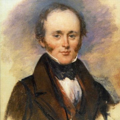
While Hutton developed the concept of uniformitarianism, Charles Lyell (1797-1875) made the idea famous in his influential book Principles of Geology, first published in 1830. Based on many observations and examples, he convinced many people that geological processes act slowly and continuously. We now know that this is not strictly true: the intensities and rates of some processes have changed over Earth’s history (for example, the interior of the Earth used to be much hotter than it is today, as it once contained much more heat-generating radioactive material) and Earth’s history has been occasionally punctuated by catastrophic events (such as the asteroid impact that sealed the fate of most dinosaurs 66 Ma). But, we still accept the uniformitarian view that the chemical and physical laws of nature have nevertheless remained constant over time.

Fundamentally, the work of Hutton and Lyell solidified the uniformitarian view that “the present is the key to the past.” This means that by studying how Earth processes work today, we can also make sense of how Earth operated in the past, as well as predict its future. Because of this, uniformitarianism is the single most important and fundamental idea in all of geology.

Principles of Relative Dating

It may surprise you to learn that geologists were able to determine much of the history of the Earth and its life without knowing anything about the actual ages of the rocks that they studied. Through use of numerical (absolute) dating techniques (which were developed during the 20th century; discussed later), they were able to later assign dates in years before present to important events in Earth’s history. But, before that, they relied upon a different approach to first determine the sequence of important events in Earth’s past: relative dating.

Relative Dating

Figure \(\PageIndex{3}\): Grand Canyon, Arizona. (CC BY-SA (https://creativecommons.org/licenses/by-sa/4.0); By Niagara66, https://commons.wikimedia.org/wiki/File:Grand_Canyon_National_Park_06.jpg.)

The principles of relative dating are largely applied to unraveling the geologic history of the thin blanket of sedimentary rock that covers much of continental land surfaces. Most of what we know about the development, diversity, and evolution of complex life is preserved in this thin blanket. The thickness of the sedimentary rock layers, or strata, varies quite a bit. In the northern Canadian Shield areas, which have been stripped clean of sedimentary cover during the past several million years of ice age glaciations, the cover is essentially zero. In locations uninterrupted by recent mountain building or the effects of glaciation, like the Gulf Coast of the United States, this cover can be substantial, up to 20 km thick (~12 miles)! The average cover is about 1800m thick (5900ft or just over 1 mile). The thickness of the sedimentary rock layers exposed in the Grand Canyon is close to the average at 1850m. This extent of visual exposure in the canyon is not found elsewhere in the U.S. which is what makes it so spectacular.

Figure \(\PageIndex{4}\): Sedimentary rock layers exposed at Quebrada de Cafayate, Salta (Argentina). (CC BY-SA 2.0, https://commons.wikimedia.org/w/inde...curid=24779211; by travelwayoflife https://www.flickr.com/photos/travelwayoflife/6164348161/in/photostream/)

The following relative dating principles apply to this covering of strata which is largely sedimentary in origin. However, igneous rock may also be included in the layers when it forms horizontally, in layers parallel to the Earth’s surface, as in lava flows, pyroclastic flows and ash falls.

Very simply, relative dating has to do with determining whether one geological or paleontological event happened before or after a second event. For example:

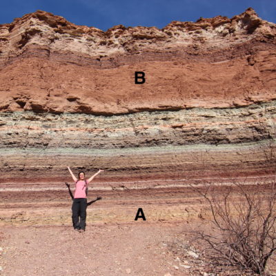
Did rock layer A form before or after rock layer B?

Did the crinoid from Indiana (below, left) live before or after the trilobite from Oklahoma (below, right)?

Figure \(\PageIndex{5}\): Fossil Trilobite. Cravat Member, Bois d’Arc formation, Lower Devonian (Held.) age, Clarita, Coal Co., Oklahoma, U.S.A. (CC BY-SA 3.0; Moussa Direct Ltd., https://commons.wikimedia.org/w/inde...?curid=4461171)

Figure \(\PageIndex{6}\): Fossil Crinoid. Agaricocrinus americanus, Carboniferous, Indiana. (CC BY-SA 3.0; https://commons.wikimedia.org/wiki/User:Vassil.)

We can answer these questions with a handful of principles that help guide our thinking when establishing how old one geologic feature is relative to another. Relative dating has to do with determining the ordering of events in Earth’s past. Geologists employ six simple principles in relative dating; the most important of which is the principle of superposition

Principle of superposition

Figure \(\PageIndex{7}\): Portrait of Nicholas Steno (public domain; Wikimedia Commons).

Nicholas Steno (1638-1686) was a well traveled Danish anatomist and one of the earliest scientists associated with studying paleontology and geology. He was the first to study relationships between layers of rock and the association of sediment, minerals and fossils to the surrounding and containing rock. He recognized the stories that rock could tell through their history of formation read as clues found within each rock. Steno’s principle of superposition is simple, intuitive, and is the basis for relative dating of geological formations. It states that rocks positioned below other rocks are older than the rocks above.

Figure \(\PageIndex{8}\): Taughannock Falls near Trumansburg, New York, illustrating the Principle of Superposition. (This work is licensed under a Creative Commons Attribution-ShareAlike 4.0 International License; Image by Jonathan R. Hendricks.)

The image to the right demonstrates this principle as it shows a sequence of Devonian-aged (~380 Ma) rocks exposed at the magnificent waterfall at Taughannock Falls State Park in central New York. The rocks near the bottom of the waterfall were deposited first and the rocks above are subsequently younger and younger. Superposition is observed not only in rocks, but also in our daily lives. Consider the trash in your kitchen garbage can. The trash at the bottom was thrown out earlier than the trash that lies above it; the trash at the bottom is therefore older (and likely smellier!).

The photograph below was captured at Volcano National Park on the Big Island of Hawaii. Use superposition to determine which is older: the road or the lava flow? How do you know?

Figure \(\PageIndex{9}\): Volcano National Park, Big Island of Hawaii. (This work is licensed under a Creative Commons Attribution-ShareAlike 4.0 International License; Image by Jonathan R. Hendricks.)

Principle of faunal succession

Figure \(\PageIndex{10}\): Sequence and correlation of fossils from different locations. (CC BY-SA; https://commons.wikimedia.org/wiki/File:Fossils.png by: Kurt Rosenkrantz)

William Smith (1769 – 1839) worked as a surveyor in the coal-mining and canal-building industries in southwestern England in the late 1700s and early 1800s. While doing his work, he had many opportunities to look at the Paleozoic and Mesozoic sedimentary rocks of the region, and he did so in a way that few had done before. Smith noticed the textural similarities and differences between rocks in different locations, and more importantly, he showed that fossils could be used to correlate rocks of the same age. Smith is credited with formulating a fundamental concept and basis for the development of the geologic time scale – the principle of faunal succession. Smith found the same ordering of fossil species from place to place; Fossil A was always found below Fossil B, which in turn was always found below Fossil C, and so on. By documenting these sequences of fossils, Smith was able to correlate rock layers (strata) from place to place. He established that rock layers in two different places were the same age based upon the fact that they include the same distinctive types of fossils.

Principle of original horizontality

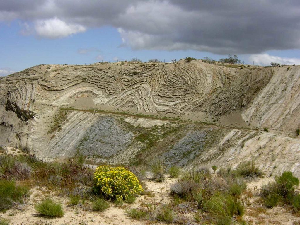
The principle of original horizontality states that sediments are deposited by gravity in layers parallel to the Earth’s surface. This applies also to volcanic igneous rocks that have been formed by lava flows, pyroclastic flows and ashfall deposits. Layers that accumulate along the edges of basins may be slightly sloped in toward the basin. This principle is particularly useful when rock layers have been deformed by the forces of tectonic activity. Students must learn to “unfold the folds” or reconstruct faulted and contorted layers that were originally horizontal to the Earth’s surface to understand their geologic history. Check out the contorted folds in the sedimentary rock layers in the photo below. From the picture it is difficult to put all the rock layers back in their originally horizontal position. A geologist would walk this area, and any adjacent areas of exposed rock layers, to make sketches, take samples and pictures and use their imagination to attempt to conceptually “unravel” the deformed layers to understand the complete story of what happened from the original deposition of sediments to get them to their current appearance.

Figure \(\PageIndex{11}\): Folds exposed in a roadcut along Highway 14 in Palmdale, California, adjacent to San Andreas fault. (With permission by: Garry Hayes and Susan Hayes from: http://geotripperimages.com/Tectonic_Processes/Folds.htm)

Principle of lateral continuity

The principle of lateral continuity states that layers of sediment initially extend outward in all directions; in other words, they are laterally continuous. As a result, rocks that are otherwise similar, but are now separated by a valley or other erosional feature (for instance, Grand Canyon), can be assumed to be originally continuous.

Layers of sediment do not extend indefinitely or infinitely. Instead, limits are controlled by the amount and type of sediment available, and the size and shape of the sedimentary basin. As sediment is transported to an area, thickest deposits are found closest to the source, and gradually thin as the distance increases.

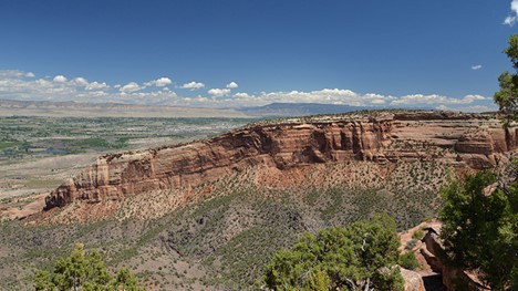
In the panoramic photo below, the originally laterally continuous layers of sedimentary rock have been cut into by the Colorado River at Dead Horse Point State Park in southern Utah.

Figure \(\PageIndex{12}\): By Jean-Christophe BENOIST (Own work, CC BY 3.0, https://commons.wikimedia.org/w/index.php?curid=10152833)

Principle of cross-cutting relationships

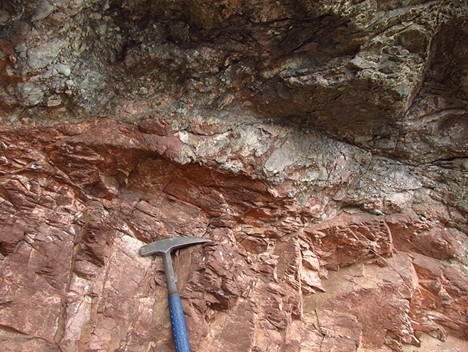
The principle of cross-cutting relationships states that any geological feature that cuts across, or disrupts, another feature must be younger than the feature that is disrupted. In the photo below, a fault disrupts the once continuous layers of sedimentary rock . The dark red “marker bed” can be used to see the displacement that has occurred on either side of the fault. The fault “cross-cuts” the layers of sedimentary rock. This indicates that the sedimentary layers pre-date the fault; the fault is the younger feature.

Figure \(\PageIndex{13}\): Normal fault offsetting layers in the Noonday Dolomite, Mosaic Canyon, Death Valley, California. (With permission by: Garry Hayes and Susan Hayes from: http://geotripperimages.com/images/DSC01776%20Normal%20fault%20in%20Mosaic%20Canyon.jpg)

Figure \(\PageIndex{14}\): Above: A thin basaltic dike cross-cutting volcanic sediments of Paleogene age at Lagganulva, on the Isle of Mull, Scotland. (By permission, John Faithful, University of Glasgow, Scotland.) Below: Feeder dike intruding tephra with basaltic lava flow above, Iceland. (By: Marli Miller from https://geologypics.com/geological_entries/gallery. For educational purposes.)

Another example of a cross cutting relationship includes an igneous intrusive feature known as a dike. In the picture to the left, hot magma forced its way into a fracture, or weakness, in pre-existing rock of the crust. The hot magma also “baked” the pre-existing rock through the process of contact metamorphism. These two clues from this exposure help us understand that the dike is younger than the rock it cross-cuts.

A final possibility occurs when a new pattern, such as tectonic cleavage or folding overprints a pre-existing structure, such as sedimentary bedding or metamorphic foliation. The pattern of folding cuts across (reconfigures) the old pattern. Here is an example from Connecticut, showing both this “overprinting” variety of cross-cutting, as well as a traditional igneous dike:

Figure \(\PageIndex{15}\): What sequence of steps were needed to make this Connecticut outcrop? (Photograph by Gregory Simones; reproduced with permission)

Figure \(\PageIndex{16}\): The sequence of steps needed to make the Connecticut outcrop. (Original photograph by Gregory Simones; reproduced with permission)

Principle of inclusions

The principle of relative dating by inclusions states that any rock fragments that are included in another body of rock must be older than the rock in which they are included. The photo below provides a good example. Both are igneous rock. The pink rock is granite while the black rock is basalt. A xenolith of the granite is included in the mass of basalt rock. How did this happen? Basalt intruded into the pre-existing pink granite. The injection of mafic magma caused a piece of the solid granite to break off, rotate a bit, and then get locked in place as an “inclusion” within the basalt as the dark magma cooled.

Figure \(\PageIndex{17}\): Included fragment (xenolith) of granite within basalt near Georgeville, Nova Scotia. (CC BY-SA 3.0; By M.C. Rygel)

Another interesting feature is apparent in this photo. The pink xenolith displays a much deeper, more rosey color which is also seen along most of the contact between the granite and basalt. This deeper, rosier color is due to the baking of the granite by the basalt. This is referred to as contact metamorphism and is also a relative dating principle. The rock that has been “baked” must have been in place prior to the intrusion of the hot magma/lava which caused the baking. You can’t cook something that doesn’t yet exist.

The following gigapixel panorama is a fascinating example of an inclusion embedded into pyroclastic ash flow deposits. The photo is from Kilbourne Hole in southeast New Mexico. The black basalt volcanic bomb was ejected during a volcanic eruption and landed in a recent pyroclastic ash flow deposit that had yet to solidify. You can easily see how this volcanic bomb deformed the layers of ash as it landed and became embedded. The lower ash layers obviously had to be there prior to the volcanic bomb landing and embedding. Later ash layers buried the bomb.

The Grand Canyon example

The Grand Canyon of the Colorado river in the U.S. state of Arizona illustrates many of the stratigraphic principles discussed thus far. The photo below shows layers of rock on top of one another in order, from the oldest at the bottom to the youngest at the top, an illustration of the principle of superposition. The predominant white layer just below the canyon rim is the Kaibab Limestone. This layer is laterally continuous with the upper white layers of strata in the far distance, even though the intervening canyon separates them. The rock layers exhibit the principle of lateral continuity, as they are found on both sides of the Grand Canyon, ten miles apart.

Figure \(\PageIndex{18}\): Many people consider Grand Canyon National Park the world’s premiere geologic landscape and a “geologic wonder”. The eroded cliffs reveal 1.7 billion years of fossils, volcanic activity, and geologic history. (United States Public Domain; National Park Service from: https://www.nps.gov/articles/age-of-rocks-in-grand-canyon.htm.)

Figure \(\PageIndex{19}\): A schematic cross-section of the strata exposed in the Grand Canyon. (United States Public Domain; Callan Bentley after National Park Service from: https://www.nps.gov/articles/age-of-rocks-in-grand-canyon.htm.)

The diagram (left) shows a cross-section of the rocks exposed on the walls of the Grand Canyon, illustrating the principle of cross-cutting relationships, superposition, and original horizontality. In the lower parts of the Grand Canyon are the oldest sedimentary formations, with igneous and metamorphic rocks at the very bottom. (For this reason, these crystalline rocks are sometimes called “the basement.”) The principle of cross-cutting relationships shows the sequence of these events. The metamorphic schist (#1) is the oldest rock formation and the cross-cutting granite intrusion (#3) is younger. As seen in the figure, the other layers on the walls of the Grand Canyon are numbered with #18 being the youngest, of all of the rocks exposed in the canyon, #18 was the last to form. This illustrates the principle of superposition. The Colorado River carves through the Colorado Plateau, exposing the horizontal strata, that follows the principle of original horizontality. These rock strata have been barely disturbed from their original deposition, except by a broad regional uplift.

Unconformities – Missing Time

An unconformity represents an interruption in the process of depositing sedimentary layers. Recognizing unconformities is important for understanding time relationships in sedimentary sequences. We can use the rock exposed in the Grand Canyon to illustrate examples of all of the different types of unconformities. Locate these on the diagram of Grand Canyon stratigraphy above as each is discussed.

Figure \(\PageIndex{20}\): The great angular unconformity in the Grand Canyon, Arizona. The tilted rocks at the bottom are part of the Proterozoic Grand Canyon Supergroup (aged 825 to 1,250 Ma). The flat-lying rocks at the top are Paleozoic (540 to 250 Ma). The boundary between the two represents a time gap of nearly 300 million years. (Credit: Doug Dolde / Doug Dolde at en.Wikipedia / Public domain. Annotated by Callan Bentley.)

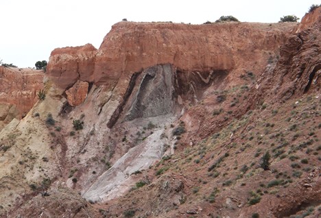
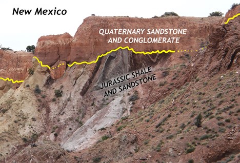
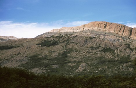
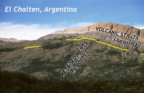
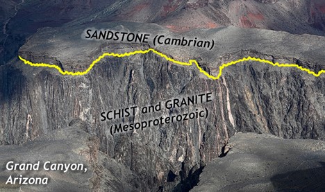
An example of one of the most iconic unconformities is shown in the lower center portion of the photo below from the Grand Canyon. It is known as “The Great Unconformity.” Proterozoic rocks of the sedimentary sequence known as the Grand Canyon Supergroup, have been tilted and then eroded to a flat surface prior to deposition of the younger Paleozoic rocks. The specific type is an angular unconformity. The difference in time between the youngest of the Proterozoic rocks and the oldest of the Paleozoic rocks is close to 300 million years. Tilting and erosion of the older rocks took place during this time, and if there was any deposition going on in this area, the evidence of it is now gone.

Figure \(\PageIndex{21}\): The view is centered on Sumner Butte, at southeast terminus of Bright Angel Canyon, intersecting with Granite Gorge. (The original uploader was Szumyk at Polish Wikipedia. – http://pdphoto.org/PictureDetail.php?mat=pdef&pg=5506, Public Domain, https://commons.wikimedia.org/w/inde...?curid=5883465. Annotated by Callan Bentley.)

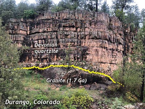
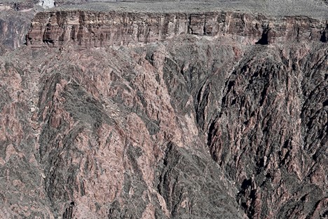
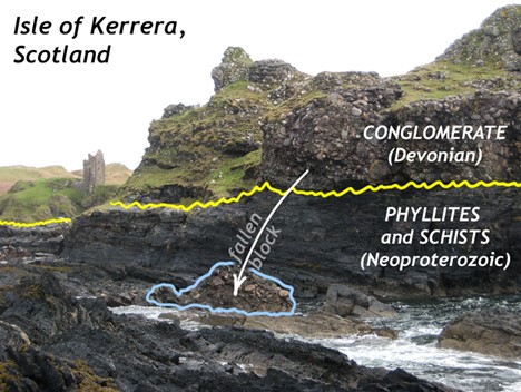
A nonconformity represents an erosional surface separating rocks of different types. The erosional surface will separate igneous and/or metamorphic rock from overlying sedimentary rock such as in the photo below, from a different spot in the Grand Canyon. In the photo, right, a nonconformity representing the erosional surface between 1.75 Ga Proterozoic age rock at the base of the Grand Canyon and ~545 Ma Phanerozoic age rock. Over 1 billion years separate the basement rock from the first overlying layer.

Figure \(\PageIndex{22}\): Redwall, Temple Butte and Muav formations in the Grand Canyon. An erosional surface (disconformity) exists between both the Muav Limestone and the Temple Butte formations as well as between the Temple Butte and the Redwall Limestone formations. (United States Public Domain; National Park Service from: https://upload.wikimedia.org/Wikipedia/commons/e/eb/Redwall%2C_Temple_Butte_and_Muav_formations_in_Grand_Canyon.jpg.)

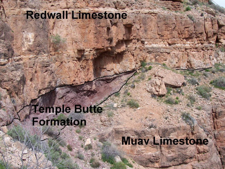
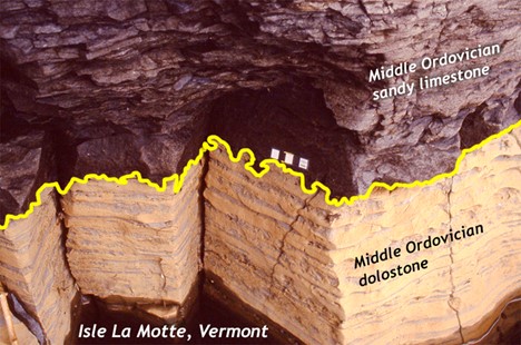
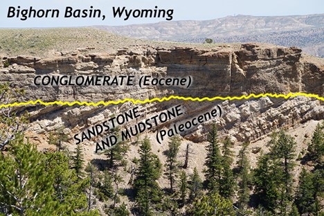
A disconformity is a little harder to discern: it is not as obvious as the previous examples. Disconformities occur between parallel sedimentary layers. Several exist in the horizontal layers of the Grand Canyon. One occurs between the Muav Limestone formation which is approximately 515 Ma and the overlying Temple Butte and Redwall Limestone formations which are approximately 350 Ma and 335 Ma, respectively. This erosional surface, representing over 150 million years is well displayed in the photo at left.

Example \(\PageIndex{1}\): Unconformity Examples

Let’s take a look at some additional examples of the different types of unconformities.

Disconformity:

Angular unconformity:

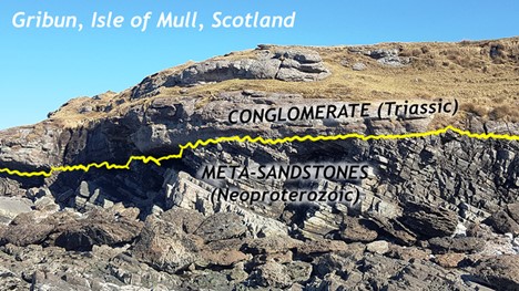
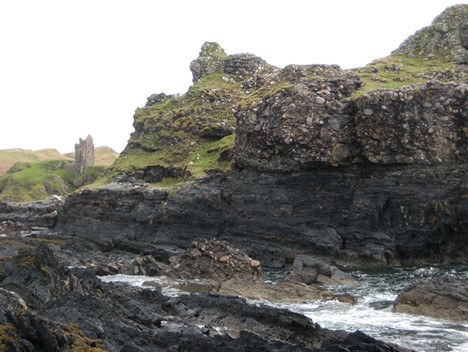
Nonconformity:

More unconformities:

Figure \(\PageIndex{23}\): Angular unconformity, Telheiro Beach, Portugal, showing Triassic sandstone atop folded, eroded, Carboniferous graywacke and shale. (Photo by Joao Duarte, 2019.)

Figure \(\PageIndex{24}\): Angular unconformity in Loughshinny, Ireland, showing flat-lying Pleistocene till overlying folded limestone and shale. (Photo by Jason Loxton, 2018.)

Figure \(\PageIndex{25}\): Angular unconformity in Loughshinny, Ireland, showing flat-lying Pleistocene till overlying folded limestone and shale of Carboniferous age. (Photo by Jason Loxton, 2018.)

Figure \(\PageIndex{26}\): Carboniferous / Cretaceous angular unconformity at Ense-Bremen, North Rhine-Westphalia, Germany. (Photo by Henning Bergermann; reproduced with permission.)

Figure \(\PageIndex{27}\): Tilted layers of Neogene-aged sandstone and shale overlain by Pleistocene gravels (with clam-bored boulder bed just above the unconformity surface). Bonus: a layer of recent colluvium overlies the gravels! (Photo by Seth Finnegan; reproduced with permission.)

Figure \(\PageIndex{28}\): Jurassic-aged Morrison Formation (shale and sandstone) folded and eroded, overlain by Quaternary sandstone and conglomerate. (Photo by Elizabeth Bollen; reproduced with permission.)

Figure \(\PageIndex{29}\): Unconformity between Neoproterozoic andesite (~570 Ma) and overlying Triassic sandstone (~210 Ma). (Photo by Jack Matthews; reproduced with permission.)

Figure \(\PageIndex{30}\): The Knox unconformity (a disconformity bounding the Sauk and Tippecanoe epeiric sequences) exposed on Isle La Motte, Lake Champlain, Vermont. Providence Island Formation of the Beekmantown Group (tidal dolomite of the Middle Ordovician) is overlain by lower Day Point Formation (also Middle Ordovician) from the Chazy Group, which is sandy limestone and carbonate sandstone. Note the karstic dissolution of the lower unit at the unconformity surface. (Photograph by Matthew Clapham; reproduced with permission.)

Figure \(\PageIndex{31}\): The “Great Unconformity” (really a nonconformity) north of Durango Colorado. 1.7 Ga Baker’s Bridge granite overlain by late Devonian Ignacio quartzite. (Photograph by Cody Mason; reproduced with permission.)

Figure \(\PageIndex{32}\): Nonconformity in Gallinas Canyon, New Mexico. (Photo by Howell Bosbyshell; reproduced with permission.)

Figure \(\PageIndex{33}\): A paleo-hill of Jurassic sandstone, overlain by Paleocene volcanics mainly basalts. It was quarried for its rock used to make the approach to a local lighthouse on the Isle of Mull. (Photo by James Westland; reproduced with permission.)

Figure \(\PageIndex{34}\): Angular unconformity at El Chalten, Argentina. Jurassic volcanic strata overlie Paleozoic meta-sedimentary strata. (Photo by Donna Anderson; reproduced with permission.)

Figure \(\PageIndex{35}\): Dipping Paleocene interbedded sands and muds with overlying horizontal Eocene conglomerates. Bighorn Basin, Wyoming. (Photo by Amanda Owen; reproduced with permission.)

Figure \(\PageIndex{36}\): Probably one of the best examples of an unconformity in Southern England. An unconformity is a buried erosional surface separating strata of different ages; it indicates that sediment deposition was not continuous. In this unconformity at the very eastern end of the Mendips, younger strata of sedimentary Jurassic Inferior Oolite rest upon the eroded surface of tilted older Carboniferous Vallis Limestone. (Reproduced via a CC-by license; Photo by Vieve Forward, https://www.geograph.org.uk/photo/4165184)

Figure \(\PageIndex{37}\): At Chippewa Falls, Wisconsin, there is an unconformity shows a \(\approx\)1.8 Ga saprolitized trondhjemite (granitoid) nonconformably overlain by the Cambrian-age Mt. Simon Sandstone. (Photo by Scott Clark; reproduced with permission.)

Figure \(\PageIndex{38}\): Pleistocene terrace deposits over Miocene Astoria Fm. The latter was deposited between episodes of Columbia River flood basalts reaching the coast, which was the case with Otter Rock, the large headland in the mid-ground. (Photo by Lockwood DeWitt; reproduced with permission.)

Figure \(\PageIndex{39}\): This is an upside-down unconformity! The rock above is ophiolitic seafloor breccia (160 Ma). The sediments at the bottom are Late Jurassic. Within the sediments there are also turbidites with inverted grading. The whole package has been flipped by tectonics (we are in the reverse limb of a major fold here). (Photo by Samuele Papeschi; reproduced with permission.)

Figure \(\PageIndex{40}\): A monocline overprinting an unconformity. Proterozoic basement rocks (purple, low in canyon) are overlain by the Chinle Formation, with the Wingate Sandstone as the cliff-forming unit. Colorado National Monument. (Photo by Robert Mahon; reproduced with permission.

Figure \(\PageIndex{41}\): Angular unconformity in the Grand Canyon. Lower tilted layers are Neoproterozoic strata of the Grand Canyon supergroup (various sedimentary rock and some lava flows). The cliff-forming unit extending horizontally across the field of view is Cambrian-aged Tapeats Sandstone. (Photo by Zoltán Sylvester; reproduced with permission.)

Figure \(\PageIndex{42}\): Pleistocene terrace deposits over deltaic deposits of the Eocene Coaledo Fm, Shore Acres State Park, Oregon. (Photo by Lockwood DeWitt; reproduced with permission.)

Figure \(\PageIndex{43}\): Nonconformity in the Grand Canyon. Lower rock unit is Mesoproterozoic schist (gray) and granite (pink). The cliff-forming unit extending horizontally across the top of the field of view is Cambrian-aged Tapeats Sandstone. (Photo by Zoltán Sylvester; reproduced with permission.)

Figure \(\PageIndex{44}\): Nonconformity in the Grand Canyon. Lower rock unit is Mesoproterozoic schist (gray) and granite (pink). The cliff-forming unit extending horizontally across the top of the field of view is Cambrian-aged Tapeats Sandstone. (Photo by Zoltán Sylvester; reproduced with permission.)

Figure \(\PageIndex{45}\): At Gribun on the Isle of Mull is an angular unconformity. The underlying dipping rocks are Neoproterozoic psammites (meta-sandstones). There are horizontal Triassic conglomerates above. Most of the boulders on the shore are the conglomerate. Higher up, but not seen in this photo, there are also Paleocene basalts. (Photo by James Westland; reproduced with permission.)

Figure \(\PageIndex{46}\): The classic Scottish angular unconformity between Dalradian metasedimentary slates/phyllites/metalimestones and the overlying basal conglomerate of Late Devonian Old Red Sandstone. This exposure is on the Isle of Kerrera. Gylen Castle ruin for scale. (Photo by Roderick Brown; reproduced with permission.)

Figure \(\PageIndex{47}\): Basal Cambrian arenites (sandstones) on Ercall Granophyre (an igneous rock, like a granite). Ercall quarries, Shropshire. (Photo by Jon Radley, University of Birmingham; reproduced with permission.)

Figure \(\PageIndex{48}\): Angular unconformity near Cody, Wyoming. The lower unit is Triassic Chugwater Formation; the upper unit is Quaternary terrace gravels. (Photo by Ben Edwards; reproduced with permission.)

Figure \(\PageIndex{49}\): A gorge in Shades State Park, Indiana shows the Mansfield Sandstone (Pennsylvanian) lying unconformly over limestones and siltstones of the Mississippian aged Borden Group. Glacial waters cut into the sandstone, creating these gorges, exposing the strata. (Photo by Troy Simpson; reproduced here with permission)

Figure \(\PageIndex{50}\): Gently dipping Triassic strata over vertical Carboniferous layers, Rainy Bay, Nova Scotia, Canada. (Photo by Jon Noad; reproduced with permission.)

Figure \(\PageIndex{51}\): 7,000-year-old Mazama Ash Bed overlying steeply dipping Carboniferous limestone. Exshaw, Alberta, Canada. (Photo by Jon Noad; reproduced with permission.)

Figure \(\PageIndex{52}\): A nonconformity exposed at Deer Creek in the Grand Canyon. The waterfall emerges from the contact between lower Mesoproterozoic basement rocks and overlying Cambrian Tapeats Sandstone. (Photo by Logan Wren Raming; reproduced with permission.)

Figure \(\PageIndex{53}\): The Kentland Disturbance Geologic Area is a theorized impact site where Ordovician and Silurian carbonate strata were forced to the surface by the impact. A quarry has existed here for a hundred years excavating rock aggregate and exposing folded and tilted strata with localized faults and telltale shattercones. The upended strata were then scraped over by Pleistocene glaciation, leaving a thin veneer of glacial deposits on top. (Photo by Troy Simpson; reproduced here with permission.)

Figure \(\PageIndex{54}\): Chapman's Drive nonconformity, with Table Mountain Group sandstones (~450 Ma) overlying Peninsula Granite (~630 Ma). Cape Town, South Africa. (Photo by Evelyn Mervine; reproduced with permission.)

Figure \(\PageIndex{55}\): Annex Hill State Park in Minnesota shows two unconformities: an angular unconformity between Archean banded iron formation and overlaying Cretaceous shale, and a disconformity between the shale and overlying Pleistocene till.

Did I Get It? - Quiz

Exercise \(\PageIndex{1}\)

What kind of unconformity is shown here?

a. nonconformity

b. disconformity

c. angular unconformity

Answer

b. disconformity

Exercise \(\PageIndex{2}\)

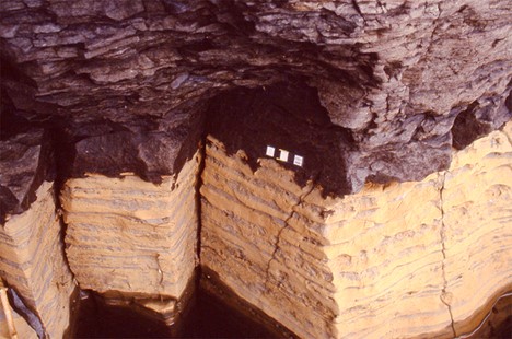
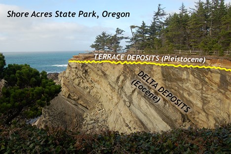
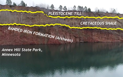
What kind of unconformity is shown here highlighted in yellow, separating black basalt over white chalk?

a. nonconformity

b. disconformity

c. angular unconformity

Answer

b. disconformity

Exercise \(\PageIndex{3}\)

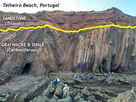
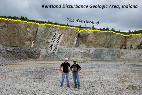
What kind of unconformity is shown here?

a. nonconformity

b. disconformity

c. angular unconformity

Answer

c. angular unconformity

Exercise \(\PageIndex{4}\)

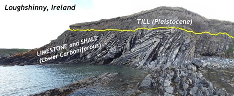
What kind of unconformity is shown?

a. nonconformity

b. disconformity

c. angular unconformity

Answer

a. nonconformity

Exercise \(\PageIndex{5}\)

What kind of unconformity is this?

a. nonconformity

b. disconformity

c. angular unconformity

Answer

a. nonconformity

Exercise \(\PageIndex{6}\)

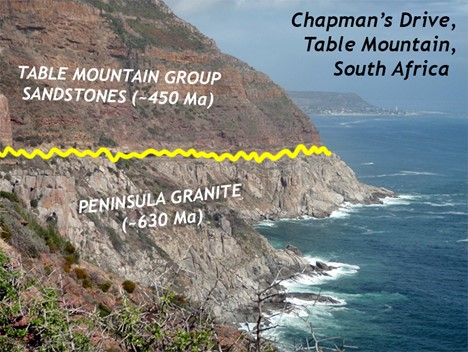
What kind of unconformity is shown here? How much time is missing?

a. This is a nonconformity. About one million years are missing.

b. This is a disconformity. About 75 billion years are missing.

c. This is an angular unconformity. About half a billion years are missing.

Answer

c. This is an angular unconformity. About half a billion years are missing.

Exercise \(\PageIndex{7}\)

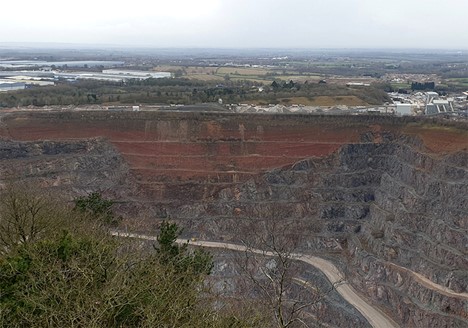
Interpret this outcrop.

a. It's a nonconformity. It implies that (1) a pluton of magma was intruded, (2) it cooled down and crystallized, (3) it was tilted up and eroded at Earth's surface, (4) a deposit of sediment was laid down, (5) it was lithified, and (6) the whole package was once again raised up to Earth's surface where we can see it (and where it is eroding anew).

b. It's a disconformity. It implies that (1) an initial deposit of sediment was laid down, (2) it was lithified, (3) it was eroded at Earth's surface, (4) a second deposit of sediment was laid down, (5) it was lithified, and (6) the whole package was once again raised up to Earth's surface where we can see it (and where it is eroding anew).

c. It's an angular unconformity. It implies that (1) an initial deposit of sediment was laid down, (2) it was lithified, (3) it was tilted up by mountain-building and eroded at Earth's surface, (4) a second deposit of sediment was laid down, (5) it was lithified, and (6) the whole package was once again raised up to Earth's surface where we can see it (and where it is eroding anew).

Answer

c. It's an angular unconformity. It implies that (1) an initial deposit of sediment was laid down, (2) it was lithified, (3) it was tilted up by mountain-building and eroded at Earth's surface, (4) a second deposit of sediment was laid down, (5) it was lithified, and (6) the whole package was once again raised up to Earth's surface where we can see it (and where it is eroding anew).

Applications of Relative Dating

Example \(\PageIndex{2}\)

Let’s take a look at an example from an exposure in Albersweiler, Germany. We usually can only capture several relative dating relationships in one picture. These relationships become much more complex in wider view or larger scale.

Figure \(\PageIndex{56}\): Geologists viewing an exposure in a quarry near Albersweiler, Germany. (Photo by: Paul R. Eizenhöfer, Eberhard Karls Universität Tübingen Germany. With permission from: https://eizenhoefer.wordpress.com/albersweilergermany)

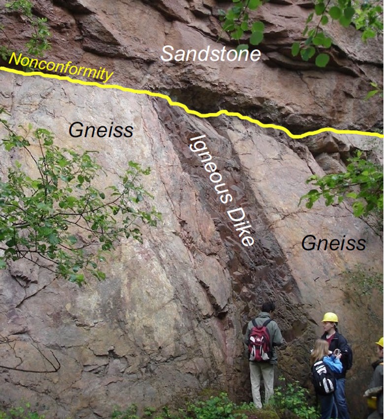
The quarry exposure displays three different rock types. From field investigation we observe the following: 1) three rock types: a grey colored gneiss, a fine grained, black igneous rock, and dark red sandstone, 2) an erosional surface between the gneiss and the overlying sandstone, 3) baking of the gneiss adjacent the the contact with the igneous rock. How can we determine the order of events?

Solution

We can use several principles above help us solve this problem. First, the principle of superposition tells us that the older rocks will be on the bottom and the younger at the top. Therefore, the gneiss is most likely older than the sandstone. The cross-cutting and baked contacts tell us that the black, igneous rock is a dike (intrusion of magma). The erosional surface at the contact between the gneiss and sandstone tells us that an unconformity exists. What type of unconformity exists between metamorphic/igneous rock and sedimentary rock? This is specifically a nonconformity. From this evidence we can conclude the following:

Oldest: gneiss, igneous dike, nonconformity, sandstone Youngest

Example \(\PageIndex{3}\)

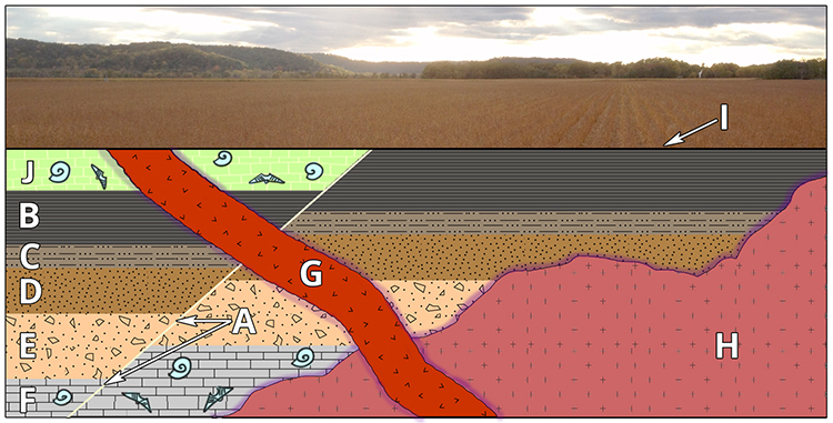
The cartoon below shows an imaginary sequence of rocks and geological events labeled A-J. Using the principles of superposition and cross-cutting relationships, can you reconstruct the geological history of this place based upon the information you have available?

Figure \(PageIndex{57}\): Relative dating relationships. (Creative Commons License. This work is licensed under a Creative Commons Attribution-ShareAlike 4.0 International License; Original image by Jonathan R. Hendricks. Modified by Callan Bentley.)

Solution

Let’s work through the imaginary example above.

First, we know from the principle of superposition that rock layer F is older than E, E is older than D, D is older than C, and C is older than B, and B is older than J.

Oldest F, E, D, C, B, J Youngest

Second, we observe that rock body H (which is an igneous intrusion) cuts into rock layers B-F, but not J. It is therefore younger than B-F and, with the data we have, we assume J as well (*), however H does not specifically cross-cut J. We can also observe the contact metamorphism “baked rim” around H so we know that B-F had to be there in order to get baked by the intrusion of H.

Oldest F, E, D, C, B, H, J* Youngest

Third, we observe that the fault A cuts across and displaces rock layers B-J. It is therefore younger than B-J. Because the fault does not cut across H, we do not know if it is older or younger than that rock unit.

Oldest F, E, D, C, B, J*, (H or A) Youngest

Fourth, we see that G, another igneous intrusion, cuts across A-J; it is therefore younger than all of these (note that G is not displaced by A, the fault).

Oldest F, E, D, C, B, J*, (H or A), G Youngest

Finally, we note an erosional surface, I, at the top of the sequence (and immediately below the corn field) that cuts both A and G. I is therefore younger than both A and G.

Putting this all together, we can determine the relative ages of these rock layers and geological events:

Oldest F, E, D, C, B, J*, (H or A), G, I Youngest

Given the information available, we cannot resolve whether H is older than A (or, vice versa). This problem could be resolved, however, if we were able to determine the age of the fossils and the also the age of the igneous intrusions. Read on!

Dating Rocks Using Fossils

Although the recognition of fossils goes back hundreds of years, the systematic cataloguing and assignment of relative ages to different organisms from the distant past—paleontology—only dates back to the earliest part of the 19th century. The oldest undisputed fossils are from rocks dated around 3.5 Ga, and although fossils this old are tiny, typically poorly preserved and are not useful for dating rocks, they can still provide important information about conditions at the time. The oldest well-understood fossils are from rocks dating back to around 600 Ma, and the sedimentary record from that time forward is rich in fossil remains that provide a detailed record of the history and evolution of life on Earth. However, as anyone who has gone hunting for fossils knows, that does not mean that all sedimentary rocks have visible fossils, or that they are easy to find. Fossils alone cannot provide us with numerical ages of rocks, but over the past century geologists have acquired enough isotopic dates from rocks associated with fossil-bearing rocks (such as igneous dikes cutting through sedimentary layers, or volcanic layers between sedimentary layers) to be able to put specific time limits on most fossils.

If we understand the sequence of evolution on Earth, we can apply knowledge to determining the relative ages of rocks. This is William Smith’s principle of faunal succession, although of course it doesn’t just apply to “fauna” (animals); it also applies to fossils of plants and other organisms.

Geologic Range

If we can identify a fossil to the species level, or at least to the genus level, and we know the time period when the organism lived, we can assign a range of time to the rock. That range might be several million years because some organisms survived for a very long time. If the rock we are studying has several types of fossils in it, and we can assign time ranges to several of them, we might be able to narrow the time range for the age of the rock considerably.

Here’s an example. Some organisms survived for a very long time, and are not particularly useful for dating rocks. Sharks, for example, have been around for over 400 million years. This is not a useful range: if you find a shark fossil in a sedimentary layer, it only tells you, “This layer is 400 million years old, or younger.” However, the great white shark has a range of 16 million years, so far, which is a much shorter amount of time. Organisms that lived for relatively short time periods are particularly useful for dating rocks, especially if they were distributed over a wide geographic area, and so can be used to compare rocks from different regions. These are known as index fossils. There is no specific limit on how short the time span has to be to qualify as an index fossil. Some lived for millions of years, and others for much less than a million years.

Figure \(\PageIndex{58}\): Geologic Range Chart. The application of bracketing to constrain the age of a rock based on several fossils. In this diagram, the colored bars represent the time range during which each of the four species (A, B, C, D) existed on Earth. Although each species lived for several million years, we can narrow down the likely age of the rock to just 700,000 years during which all four species coexisted. (CC BY 4.0; Steven Earle. From: https://opentextbc.ca/physicalgeolog...using-fossils/)

A geoscientist can also date rocks using the geologic ranges of an fossil assemblage from a single sedimentary layer. A fossil assemblage (or faunal assemblage) is a group of organisms that all found fossilized together in that layer. This application involves the bracketing of overlapping ranges to constrain the age of a rock based on several fossils. Consider the diagram left–four species of fossils (A, B, C, D) were collected from one stratum. The geologic ranges of each species are plotted side by side in a geologic range chart. Although each species lived for several million years, we can narrow down the likely age of the rock to just 700,000 years during which all four species coexisted. Comparison of these geologic ranges shows only a short time interval (from 7-7.7 Ma) when all four species overlap. Therefore, the age of the sedimentary layer from which these fossils were collected is constrained to the interval when all four species coexist.

Biozones

Some well-studied groups of organisms qualify as biozone fossils (a stratigraphic interval that can be defined on the basis of a specific fossil) because, although the genera and families lived over a long time, each species lived for a relatively short time and can be easily distinguished from others on the basis of specific features. For example, ammonoids have a distinctive feature known as the suture line—where the internal shell layers (septae) that separate the individual chambers meet the outer shell wall. These suture lines are sufficiently variable to identify species. These can be used to estimate the age of the rocks in which they are found. Generally, the more complex the suture pattern, the younger the fossil. Compare the sutures in the following fossil specimens. The fossil ammonoid on the left is Triassic in age, specifically living in the range between 251-237 Ma. The fossil ammonoid on the right is Cretaceous in age, specifically living in the range between 113-100 Ma. Select the play button to explore these fossils in 3D.

Figure \(\PageIndex{59}\): Fossil specimen of the ceratite ammonoid Gymnotoceras beachi from the Triassic Toad Formation of British Columbia (PRI 43629). Specimen is from the collections of the Paleontological Research Institution. Maximum diameter is approximately 4.5 cm. (CC0 Public Domain; Model by Emily Hauf.)

Figure \(\PageIndex{60}\): Fossil specimen of the ammonoid cephalopod Cleoniceras besairiei from the Cretaceous period. Specimen is from the collections of the Paleontological Research Institution, Ithaca, New York. Maximum diameter of specimen is approximately 12 cm. (CC0 Public Domain; Model by Emily Hauf.)

Foraminifera are small, carbonate-shelled marine organisms that originated during the Triassic and are still around today. They are extremely useful biozone fossils. As shown in the figure below, numerous different foraminifera lived during the Cretaceous. Some lasted for over 10 million years, but others for less than 1 million years. If the foraminifera in a rock can be identified to the species level, we can get a good idea of its age. The following is an abbreviated geologic time scale displaying select index foraminifera and age range from the Cretaceous and Paleogene time periods. The gigapixel photo that follows is of Cribratina texana, collected at “Fossil Hill,” near the Chihuahua (Mexico) / Texas / New Mexico triple point border. Being that this is an index fossil, we can accurately date the age of the rock that hosts the fossil as being between 112-93.5 Ma.

Figure \(\PageIndex{61}\): Select index foraminifera from the Cretaceous and Paleogene. (For educational purposes from the Geologic Timescale Foundation, https://timescalefoundation.org/. Modified by Shelley Jaye.)

Figure \(\PageIndex{62}\): Fossils of the benthic foraminiferid Cribratina, an index fossil for the Albian-Cenomanian age, collected at “Fossil Hill,” north of the Cristo Rey laccolith at the Chihuahua (Mexico) / Texas / New Mexico triple border. (Robin Rohrback, Mid-Atlantic Geo-Image Collection (M.A.G.I.C.).)

Watch this video to learn about the discovery of conodonts and their use as index fossils.

Numerical (or Absolute) Dating

Numerical (also known as absolute) dating deals with assigning actual dates (in years before the present) to geological events. Contrast this with relative dating, which instead is concerned with determining the order of events in Earth’s past. The science of absolute age dating is known as geochronology and the fundamental method of geochronology is radiometric dating (also known as isotopic dating).

Figure \(\PageIndex{63}\): Archbishop James Ussher (1581-1656) (public domain; WikiMedia Commons).

Scholars and naturalists, understandably, have long been interested in knowing the absolute age of the Earth, as well as other important geological events. In 1650, Archbishop James Ussher (1581-1686) famously used the genealogy of the Old Testament of the Bible (e.g., Genesis, Chapter 5), and the human lifespans recorded in it, to estimate the age of the Earth. He concluded that the Earth was young in age, having formed in 4004 B.C., or about 6,000 years ago.

In the 1800’s, practitioners of the young science of geology applied the uniformitarian views of Hutton and Lyell (discussed earlier in this chapter) to try to determine the age of the Earth. For example, some geologists observed how long it took for a given amount of sediment (say, a centimeter of sand) to accumulate in a modern habitat, then applied this rate to the total known thickness of sedimentary rocks. When they did this, they estimated that the Earth is many millions of years old.

We now know that this estimate is far, far too young. In part, this estimate is so low because these early geologists did not recognize that unconformities, which represent missing units of time, often caused by erosion, are rampant in the rock record, as well as the fact that some metamorphic rocks were once sedimentary, and thus left out of their calculations. Still, this estimate was on the order of millions of years, rather than Ussher’s calculation of 6,000. Geologists were beginning to accept the views of Hutton that the Earth is unimaginably ancient.

What key discovery, then, allowed geologists to begin assigning absolute age dates to rocks and ultimately discover the age of the Earth? The answer is radioactivity.

Radiometric dating

Hypotheses of absolute ages of rocks (as well as the events that they represent) are determined from rates of radioactive decay of some isotopes of elements that occur naturally in rocks.

ELEMENTS AND ISOTOPES

In chemistry, an element is a particular kind of atom that is defined by the number of protons that it has in its nucleus. The number of protons equals the element’s atomic number. Have a look at the periodic table of the elements below. Carbon’s (C) atomic number is 6 because it has six protons in its nucleus; gold’s (Au) atomic number is 79 because it has 79 protons in its nucleus.

Figure \(\PageIndex{64}\): The periodic table of the elements of the world, showing element names, oxidation states, electron negativities, first ionization energies, and electron configurations. (CC0 1.0 Universal; Public domain from Wikimedia)

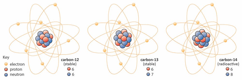
Even though individual elements always have the same number of protons, the number of neutrons in their nuclei sometimes varies. These variations are called isotopes. Isotopes of individual elements are defined by their mass number, which is simply the number of protons + the number of neutrons.

Consider, for example, the three different isotopes of Carbon:

• Carbon-12 (\(^{12}\)C): 6 protons, 6 neutrons
• Carbon-13 (\(^{13}\)C): 6 protons, 7 neutrons
• Carbon-14 (\(^{14}\)C): 6 protons, 8 neutrons

Figure \(\PageIndex{65}\): The three isotopes of carbon. (CC-ND 2.0; Tessa Koumoundouros from: https://theconversation.com/explainer-what-is-an-isotope-10688.)

RADIOACTIVE DECAY

Figure \(\PageIndex{66}\): Decay chain of U-238 to stable Pb-206. (Creative Commons Attribution-NonCommercial-ShareAlike 4.0 International License; Salt Lake Community College, An Introduction to Geology, from: http://opengeology.org/textbook/7-geologic-time/#721_Radioactive_Decay/.)

Most isotopes are stable, meaning that they do not change, or decay, over time; they could remain the same stable isotope for eternity. Some isotopes, however, are unstable and undergo radical change through the process of radioactive decay. This involves the unstable isotopes shedding energy in the form of radiation and subatomic particles, causing their numbers of protons and neutrons to change. Once the number of protons change, the isotope is no longer the same element. The radioactive element will decay to form a different, stable element. The atomic nucleus that undergoes radioactive decay is known at the parent and the resulting stable element, the daughter product (or, decay product). Consider the example of the radioactive element \(\ce{^{238}U}\) (Uranium-238) which will radioactively decay to \(\ce{^{206}Pb}\) (Lead-206). This is not a one step process as indicated in the diagram below. We begin with \(\ce{^{238}U}\) in the upper left. As the decay process releases particles and energy, \(\ce{^{238}U}\) goes through a significant transformation, morphing into many other similarly radioactive elements prior to ending up as a stable isotope of lead, \(\ce{^{206}Pb}\). Some steps take only fractions of a second, others may take thousands of years, however, relative to the pace of “geologic time,” this process happens very quickly.

How do we apply the radioactive decay of unstable isotopes to the dating of rock? We are not really dating the rock, we are dating a mineral in the rock. Radioactive elements become part of the mineral chemistry during the crystallization process. The key to understanding how this works is to realize that the physical chemistry of a growing mineral crystal can be ‘picky’ or it can be ‘sloppy.’ When ‘picky’ minerals are forming, their growing mineral crystal lattice can be very “exclusive” about what atoms it will let into its crystal structure. It accepts a select few kinds of atoms, but turns away most every other kind. The opposite would be sloppy – where all sorts of different atoms are permitted into the developing lattice. Sloppy minerals aren’t going to be useful for geologic dating. We need picky minerals.

The ideal mineral for numerical dating accepts some atoms into its crystal that are radioactive parent isotopes. The parent will decay at a known rate, diminishing in number over time but causing their daughter (decay) products to accumulate over time in a one-for-one match. The ideal mineral loves bringing in the parent, but would never include the daughter in the developing crystal structure – like a “no children allowed” rule!

In some cases, the radioactive element in question is an isotope of an element essential to the mineral’s growth; one of its “standard ingredients” – for instance, \(\ce{^{40}K}\) getting incorporated into the ‘potassium spot’ in the potassium feldspar crystal (\({\bf{\ce{K}}}\ce{AlSi3O8}\)), where most of the atoms in that position are stable (not radioactive) isotopes of the same element, \(\ce{^{39}K}\) or \(\ce{^{41}K}\) in this case. \(\ce{^{40}K}\) is the radioactive parent. \(\ce{^{40}K}\) will decay to form \(\ce{^{40}Ar}\) as a stable daughter product. However, \(\ce{^{40}Ar}\), due to its size, will never be found in the original mineral. As radioactive decay of \(\ce{^{40}K} \rightarrow \ce{^{40}Ar}\) transpires over time, both elements remain trapped within the closed system of the formed mineral.

In other cases, we’re focused on elemental impurities in the mineral crystal – atoms you won’t find in the mineral’s common chemical formula. Specifically, picky minerals will (a) let certain radioactive atoms into their crystals, but (b) at the same time, they actively exclude the stable daughter atoms that result when the radioactive parents break down. The parent isotope “fits” into the crystal, by virtue of its valence state and its atomic size. Conversely, the daughter isotope doesn’t fit into the crystal, either because of its valence state or because of its atomic size, or both. An example of this occurs in the mineral zircon (\(\ce{ZrSiO4}\)). Stable atoms of Zr dominate in the crystal lattice however radioactive \(\ce{^{238}U}\) atoms can substitute for Zr. The daughter product of the decay of \(\ce{^{238}U}\) is \(\ce{^{206}Pb}\). Due to the atomic characteristics of Pb, there is no “happy place” for Pb in the crystal, so Pb atoms will never enter the zircon crystal lattice while it is forming. As radioactive decay of \(\ce{^{238}U} \rightarrow \ce{^{206}Pb}\) occurs over time, both elements remain trapped within the closed system of the formed mineral.

The parent-daughter decay pair found within the mineral crystal starts off with 0% daughter isotopes, and 100% radioactive parent isotopes. Based on the previous discussion, we can be confident that any daughter isotopes we find in the mineral crystal got there due to radioactive decay of a parent isotope some time after the crystal originally formed, and they were NOT there from the very beginning. They form in place, due to the spontaneous breakdown of their radioactive parent isotopes, and they are “trapped” in a mineral crystal in which they do not belong. A comprehensive count of all the parent isotopes and all the daughter isotopes in that mineral system will sum to 100%.

Minerals that meet these criteria are very few and far between. The most applicable ones are listed below on the Half-life Decay Constant Chart.

HALF-LIFE DECAY CONSTANT CHART

Table \(\PageIndex{1}\): Half-Life Decay Constant Chart.

Mineral	Radioactive parent that is “allowed” in the crystal	Daughter isotope that results	Half-life decay constant of the parent isotope	Useful age range in geologic dating	Useful in Igneous rocks	Useful in Sedimentary rocks	Useful in Metamorphic rocks
Zircon (also Monazite)	\(\ce{^{238}U}\)	\(\ce{^{206}Pb}\)	4.5 billion years	More than 100 Ma	\(\checkmark\)	\(\checkmark\)*	\(\checkmark\)**
	\(\ce{^{235}U}\)	\(\ce{^{207}Pb}\)	703.8 million years	More than 100 Ma	\(\checkmark\)	\(\checkmark\)*	\(\checkmark\)**
	\(\ce{^{232}Th}\)	\(\ce{^{208}Pb}\)	14 billion years – longer than the age of the Universe!	More than 200 Ma	\(\checkmark\)	\(\checkmark\)*	\(\checkmark\)**
Muscovite, biotite, hornblende, potassium feldspar	\(\ce{^{40}K}\)	\(\ce{^{40}Ar}\)	1.25 billion years	More than 100,000 years	\(\checkmark\)		\(\checkmark\)
Muscovite, biotite, potassium feldspar	\(\ce{^{87}Rb}\)	\(\ce{^{87}Sr}\)	48.8 billion years ~4 times older than the age of the Universe!	More than 100 Ma	\(\checkmark\)		\(\checkmark\)?

*as detrital grains within a sedimentary deposit: gives a maximum age for the deposit.
**as overgrowths on original grains – must be distinguished from the mineral’s “core” during the dating process or as reset ages, if the rock has undergone very hot metamorphism (>800 \(^{\circ}\)C).

Did you notice how few minerals there are? Of the thousands of minerals known, only a handful are common enough in rocks and ‘picky’ enough in their chemistry to be useful for isotopic dating. Our toolbox has only about a dozen tools in it. We can’t numerically date quartz. We can’t numerically date calcite. Same for olivine and pyroxene and most of the important rock forming minerals.

Two pieces of information are needed to calculate how old a given mineral is: the ratio of parent to daughter isotopes, and the rate of decay, or half-life, of the radioactive parent.

• The ratio of parent to daughter atoms is measured by using a mass spectrometer which is a very sensitive, high precision instrument that detects and separates atoms based on their mass.
• The rate at which a particular parent isotope decays into its daughter product is constant. This rate is determined in a laboratory setting. A half-life is the amount of time needed for half of the parent atoms in a sample to decay into daughter products. This is illustrated in the chart below.

Figure \(\PageIndex{67}\): Radioactive Decay Curve diagram. Relationship between the amount of radioactive parent atoms in a sample relative to the number of daughter atoms over the passage of time, measured in half-lives. (This work is licensed under a Creative Commons Attribution-ShareAlike 4.0 International License; Image by Jonathan R. Hendricks.)

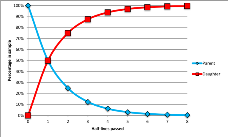
At the start time (zero half-lives passed), the sample consists of 100% parent atoms (blue diamonds); there are no daughter products (red squares) because no time has passed. After the passage of one half-life, 50% of the parent atoms have become daughter products. After two half-lives, 75% of the original parent atoms have been transformed into daughter products (thus, only 25% of the original parent atoms remain). After three half-lives, only 12.5% of the original parent atoms remain. As more half-lives pass, the number of parent atoms remaining approaches zero.

The ratio of parent atoms relative to daughter products in a sample will determine how many half-lives have passed since a mineral grain first formed. Consider the example shown below.

Figure \(\PageIndex{68}\): An example of how the initial number of radioactive parent atoms (blue diamonds) in two mineral grains (gray hexagons) changes over time (measured in half-lives) relative to the number of daughter products (red squares). (This work is licensed under a Creative Commons Attribution-ShareAlike 4.0 International License; Image by Jonathan R. Hendricks.)

The left-most box in the figure above represents an initial state, with parent atoms distributed throughout molten rock (magma). As the magma cools, grains of different minerals begin to crystalize. Some of these minerals (represented above as gray hexagons) incorporate the radioactive parent atoms (blue diamonds) into their crystalline structures; this marks the initiation of the “half-life clock” (i.e., the start time, or time zero). After one half-life has passed, half (50%, or four) of the parent atoms in each mineral grain have been transformed into their daughter products (red squares). After two half-lives have passed, 75% (six) of the original parent atoms in each grain have been transformed into daughter products. How many parent atoms would remain if three half-lives passed?

CALCULATING RADIOMETRIC DATES

The next step in radiometric dating involves converting the number of half-lives that have passed into a numerical (i.e., absolute) age. This is done by multiplying the number of half-lives that have passed by the half-life decay constant of the parent isotope (see the table above for decay constants).

Let’s step through a simple problem to determine the age of the sample of granite below.

Granite contains the mineral potassium feldspar which can be dated using the radioactive decay pair of \(\ce{^{40}K} \rightarrow \ce{^{40}Ar}\) [2] We send our sample of potassium feldspar off to the lab to be analyzed using the latest mass spectrometry methods to determine the ratio of parent isotope of \(\ce{^{40}K}\) to daughter isotope of \(\ce{^{40}Ar}\). Analysis reveals that 75% of our parent \(\ce{^{40}K}\) remains and 25% of our daughter is present. We can use the half life chart (above) and the graph below to determine the age of the granite. The chart tells us that the half life of \(\ce{^{40}K}\) is 1.25 billion years. We read the graph as follows:

Figure \(\PageIndex{69}\): Radioactive Decay Curve Half Life Plot – example problem.

We can use either the percentage of the parent or the daughter; we will end up with the same answer. Choosing the daughter percentage of 25%, we find that along the left, vertical axis and then determine the intersection with the decay curve line for the daughter product (A). We drop down vertically from that point to the horizontal axis of half lives (B). The intersection of line B with the horizontal axis indicates that approximately 0.4 of one half life has passed since this sample originally formed. To determine the age of the sample in years, we simply multiply the half life decay constant for \(\ce{^{40}K} \rightarrow \ce{^{40}Ar}\) (1.25 By) by the number of half-lives passed (0.4):

\[1.25 \text{ By X } 0.4 = 500 \text{ My}\nonumber\]

To summarize, to determine the age of a sample you must:

1. Determine the percent of Parent/Daughter isotopes that exist within the sample.

2. Determine the number of half-lives that have passed by using the percent parent (or daughter) isotope and the Radioactive Decay Curve diagram.

3. Determine the age of the sample by multiplying the number of half-lives by the decay rate constant for the parent/daughter isotope pair found on the Half-life Decay Constant chart.

A WORD ABOUT CARBON-14 (\(\ce{^{14}C}\)) DATING

Almost everyone has heard of Carbon-14 dating. \(\ce{^{14}C}\) does not appear on our Half-life Decay Constant chart above because it is not a useful isotope for dating rocks. \(\ce{^{14}C}\) has a very short half-life, geologically speaking. Its half-life is 5,730 years; compare that with the half-life data on the chart. After 5-6 half-lives (approximately 50,000 years), the amount of \(\ce{^{14}C}\) remaining is a sample becomes negligible and not useful for mineral/rock dating purposes. Carbon commonly exists in rock in the form of organic carbon and carbonate fossils. However the formation of lithified rock is in the order of millions of years therefore, any \(\ce{^{14}C}\) that originally existed in the sample has long since decayed to virtually nothing. As a result, \(\ce{^{14}C}\)’s main use is determining archeological dates of wood, charcoal, seeds, pollen, pottery, paper, natural fabric and more recent bone and shell material.

MINERAL AGES VS. ROCK AGES

How does the mineral’s numerical date relate to the rock’s numerical date? What considerations must the historical geologist bear in mind as they make the transfer from the one to the other? It depends on the rock, and it depends on the mineral.

The simplest case is with igneous rocks, wherein all the minerals form at the time molten rock (magma or lava) crystallizes into solid rock. Bowen’s crystallization sequence aside, this is more or less “instantaneous” from the perspective of most Historical Geology questions. So in igneous rocks, all the minerals are the same age as the rock. A zircon crystal (igneous mineral) date from a granite (igneous rock), therefore, may be taken as representative of the age of the granite. Exceptions would include xenoliths (pieces of older rock incorporated into igneous rocks) and xenocrysts (crystals from older rocks incorporated into igneous rocks).

In a clastic sedimentary rock, however, the situation is more complicated. Rocks like sandstone are made of sedimentary grains: small pieces of other rocks. Those other rocks must be older, in order to slough off pieces of themselves; pieces that can later be deposited with other small rock chunks and make a deposit of sand, sand that could then be lithified to make a sandstone. The minerals that make up a clastic sedimentary rock don’t form in place: they originated elsewhere, some time before. So a zircon crystal in a sedimentary rock does not represent a maximum age for the sedimentary deposit: its age is the age of the igneous rock in which it formed, so the sedimentary deposit which contains a bit of rock weathered out of that original igneous rock must be younger than it. If the zircon is 2 billion years old, then the sedimentary deposit containing it must be younger than 2 billion years old. But it could be 1 billion years old, or 100 million, or 100 years old. It could be 20 minutes old, and still contain a 2-billion-year-old zircon.

Figure \(\PageIndex{70}\): Quartz-pebble metaconglomerate (Jack Hills Quartzite), the rock type that contains the Earth’s oldest dated mineral grains (detrital zircon). (CC BY 2.0; James St. John – Quartz-pebble metaconglomerate (Jack Hills Quartzite, Archean, 2.65 to 3.05 Ga; Jack Hills, Western Australia))

These are called “detrital zircons” to distinguish our understanding of how they got into the sedimentary rock – they are survivors from older weathered-away igneous source rocks. They are part of the leftover scraps – the detritus, or waste – from the breakdown of older rocks. Detrital zircon have been very useful in tracking down the Earth’s oldest rocks. At the beginning of this chapter, you learned that the Earth is 4.56 billion years old. As it turns out, the oldest dated mineral–a grain of zircon from the Jack Hills of Western Australia–is 4.404 billion years old. This zircon exists in metaconglomerate, a metamorphosed clastic sedimentary rock. Discovery of the age of this zircon tells us that it was derived from even older igneous rock which gives us a tremendous clue as to the composition of Earth’s early, Hadean age, crust.

In a chemical sedimentary rock, where crystals are forming at the time of deposition, it would be plausible that a mineral date could be used to date the depositional age, but the problem is that none of the crystals in chemical sedimentary rocks are “picky” enough about their isotopic inclusions for the technique to work. Calcite doesn’t grab radioactive isotopes while excluding their daughter isotopes, and neither does halite or gypsum. Tough luck: we just can’t date chemical sedimentary rocks using such a process. Next!

With metamorphic rocks, there’s another layer of complication still: the mineral age can be representative of the rock’s protolith, or the date of its metamorphism. It all depends on what mineral we’re talking about, and what the protolith was. First, let’s consider a metavolcanic rock – a metamorphic rock that started off as a volcanic (igneous) rock before it got metamorphosed. In this case, a zircon represents the age of the protolith (the age of the initial eruption), while the elevated temperature and pressure of metamorphism might encourage the growth of new metamorphic minerals. When a basalt is metamorphosed to make an amphibolite for instance, it grows new amphibole crystals. These amphiboles could be dated (using the K/Ar technique) in order to determine the age of metamorphism. Two minerals in one rock, each representative of a different process, happening at a distinct time. The careful geologist should pay attention to which mineral they are dating, and what its implications are for the history of that rock.

Next, consider a metasedimentary rock – a metamorphic rock with a sedimentary protolith. A metagraywacke is a metamorphosed graywacke: its protolith was clay-rich sandstone. In this case, a detrital zircon might well be a maximum age constraint of the original sedimentary deposit, as we just discussed a couple of paragraphs ago. Zircon has a very high closure temperature (link to resetting discussion below), so if the metamorphism was low- to medium-grade, the zircon’s original igneous date could survive heating. But the same level of metamorphism in the same metagraywacke could easily be sufficient that the clay all recrystallizes to make muscovite mica, then we can use the mica to get the age of metamorphism. The zircon would have been there before metamorphism, but the mica grew as a consequence of metamorphism. Muscovite can be dated using K/Ar dating, or its derivative technique, Ar/Ar dating (link).

An example of this can be found in the Piedmont metamorphic rocks of Washington, DC. There, detrital zircons in metagraywackes of the Sykesville Formation give U/Pb ages of ~1 Ga, but the same rocks also host metamorphic muscovites that grew at 460 Ma, according to the K/Ar dating technique. The conclusion is that the muddy sand was deposited sometime after 1 Ga, but before 460 Ma, since it was metamorphosed then. The two dating techniques, on two different minerals, help “bracket” the age of the original deposit of sediment.

Figure \(\PageIndex{71}\): SHRIMP allowed in situ dating of discrete zones in zircon. This revealed for the first time the true complexities of the geochronology of this mineral as well as its ability to record individual geological events. (With permission from the Research School of Earth Sciences, Australian National University College of Science, http://shrimp.anu.edu.au/shrimp/history.php)

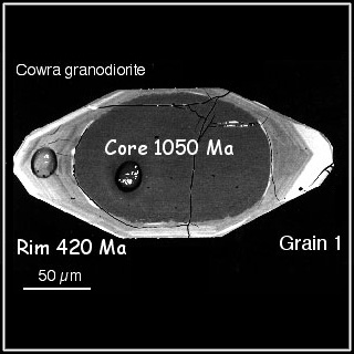
One additional wrinkle with metamorphic rocks is that sometimes you can get several dates out of a single mineral crystal. This happens because an original crystal can add new layers when it gets metamorphosed. Again, we turn to zircon for an example: if a granite pluton was to be metamorphosed and make a gneiss, then original (igneous) zircons in the rock might have the opportunity to acquire new zirconium, silicon, and oxygen atoms through metamorphic recrystallization. These new atoms get arranged in the zircon’s distinctive crystal structure, accumulating on the outside of the old crystal. If you were to date this whole zircon crystal, you’re going to get a hybridized age – a mix of the original plutonic age and the age of the metamorphic overgrowth. That would be a disaster!

Fortunately, there is a solution: SHRIMP to the rescue! SHRIMP is an acronym that stands for Sensitive High-Resolution Ion MicroProbe. It’s a tool that allows the dating of different parts of a single zircon crystal. Although the crystal being examined may be the size of a grain of sand, the SHRIMP uses a thin laser beam to distinguish between the layers on the edge (youngest) versus the layers in the middle (oldest). Incredibly, this allows us to extract multiple dates from a single mineral grain: one date for the igneous crystallization, and another date for a later metamorphic event. There are even examples where 10 or more dates have been extracted from a single grain of zircon!

Metamorphism can complicate accurately dating the age of a particular mineral. Increased pressure and temperature during metamorphism plus the addition/liberation of fluids and gases can result in ions becoming mobile in the metamorphic environment. We can return to a previous discussion on calculating radiometric dates to use as an example. Potassium feldspar is one of the most common minerals in the crust; common in both igneous and metamorphic rocks. Potassium feldspar typically begins its existence as a mineral formed during the crystallization of magma. It is a common constituent in the igneous rock, granite. The radioactive isotope, \(\ce{^{40}K}\), can be included in the crystalline structure of potassium feldspar. Upon crystallization, the radioactive decay of \(\ce{^{40}K}\) begins producing \(\ce{^{40}Ar}\). Granite can be very accurately dated using this decay pair (\(\ce{^{40}K} / \ce{^{40}Ar}\)). However, most granite is exposed to metamorphic conditions because it typically forms in a cooling magma chamber, deep within the crust, in a tectonic environment that includes the compressive forces of plate collision. Granite, subjected to metamorphic conditions, does not change much in its mineralogy however the increased pressure and temperature conditions will realign minerals and allow trapped fluids and gasses to escape. The resulting metamorphic rock is a granitic gneiss. The realigned potassium feldspar minerals will remain in the granitic gneiss (see photo below) and still contain the decaying \(\ce{^{40}K}\). However, the daughter product, \(\ce{^{40}Ar}\), formed in the original granite, may have vacated the closed system during the metamorphic process thereby resetting the radiometric decay clock. Dating the potassium feldspar in the granitic gneiss would yield the date of metamorphism, not the original date potassium feldspar crystallization in the granite.

Figure \(\PageIndex{72}\): A comparison of granite and gneiss. The texture of the protolith granite is the same in every direction (equigranular) but the gneiss has a pronounced foliation, which we infer to have developed from squeezing (compressional stress) in a direction that was perpendicular to the resulting foliation.

Applications of all dating methods

Let’s return to our Relative Dating cartoon to see how we can apply all relative and numerical dating methods to further our understanding of events in geological history. To summarize from our relative dating analysis above, here is what we know:

Oldest F, E, D, C, B, J*, (H or A), G, I Youngest. From the data given we could not tell the exact order in which fault A or igneous intrusion H occurred. We also assume* that F through J were in place prior to the intrusion of H however we do not know that since H does not cross-cut J.

Figure \(\PageIndex{73}\): Relative dating relationships. Original image by Jonathan R. Hendricks. (This work is licensed under a Creative Commons Attribution-ShareAlike 4.0 International License. Modified by Callan Bentley.)

We observe that there are fossils in both limestone units F and J. Using the principle of faunal succession and the paleontological tool of the fossil record we determine that a specific type of brachiopod fossil in layer F is from the genus Mucrospirifer. This brachiopod is an index fossil for the Devonian period during the Paleozoic Era of geologic time. Layer J reveals a cephalopod fossil from the genus Domatoceras. The geologic range for this fossil is the Pennsylvanian-Permian periods of the Paleozoic Era. We can add the following to our sequence of events:

Oldest F (Devonian), E, D, C, B, J* (Pennsylvanian-Permian), (H or A), G, I Youngest

The igneous intrusions G and H can provide us with numerical dates using isotopic analysis and our learned radiometric dating techniques. We will say that intrusion H is granite and intrusion G is basalt. The granite was analyzed using zircon crystals and the \(\ce{^{238}U/ ^{206}Pb}\) isotopes which provided an age of 330 Ma +/- 5 Ma. The basalt was analyzed using \(\ce{^{40}K} / \ce{^{40}Ar}\) of hornblende crystals yielding an age of 220 Ma +/- 8 Ma. Using the geological time scale below, we discover that the igneous intrusion H occurred during the Mississippian Period and G occurred during the Triassic Period. That provides us with some much needed timing from which we can now determine the sequence of all events.

Oldest F (Devonian), E, D, C, B, H (Mississippian), J (Pennsylvanian-Permian), G (Triassic), I Youngest

From this information can we now determine when Fault A occurred? Yes, we can!

Since Fault A cross-cuts J, we know that J is older than A. However, the intrusive dike G cross-cuts everything so we know that A is older than G. I is the erosional surface so it is the absolute youngest. So now, using all of our dating methods we can emphatically put all of the events in order:

Oldest F, E, D, C, B, H, J, A, G, I Youngest

Unraveling geologic events is a puzzle. Geologists find new pieces to the puzzle of Earth every day and continue to add pages to the book of our natural history. You can challenge yourself on a similar example in this case study: Extremadura.