
1.3: Calculations of TOA radiance and TOA reflectance
- Page ID
- 17274

\( \newcommand{\vecs}[1]{\overset { \scriptstyle \rightharpoonup} {\mathbf{#1}} } \)
\( \newcommand{\vecd}[1]{\overset{-\!-\!\rightharpoonup}{\vphantom{a}\smash {#1}}} \)
\( \newcommand{\id}{\mathrm{id}}\) \( \newcommand{\Span}{\mathrm{span}}\)
( \newcommand{\kernel}{\mathrm{null}\,}\) \( \newcommand{\range}{\mathrm{range}\,}\)
\( \newcommand{\RealPart}{\mathrm{Re}}\) \( \newcommand{\ImaginaryPart}{\mathrm{Im}}\)
\( \newcommand{\Argument}{\mathrm{Arg}}\) \( \newcommand{\norm}[1]{\| #1 \|}\)
\( \newcommand{\inner}[2]{\langle #1, #2 \rangle}\)
\( \newcommand{\Span}{\mathrm{span}}\)
\( \newcommand{\id}{\mathrm{id}}\)
\( \newcommand{\Span}{\mathrm{span}}\)
\( \newcommand{\kernel}{\mathrm{null}\,}\)
\( \newcommand{\range}{\mathrm{range}\,}\)
\( \newcommand{\RealPart}{\mathrm{Re}}\)
\( \newcommand{\ImaginaryPart}{\mathrm{Im}}\)
\( \newcommand{\Argument}{\mathrm{Arg}}\)
\( \newcommand{\norm}[1]{\| #1 \|}\)
\( \newcommand{\inner}[2]{\langle #1, #2 \rangle}\)
\( \newcommand{\Span}{\mathrm{span}}\) \( \newcommand{\AA}{\unicode[.8,0]{x212B}}\)
\( \newcommand{\vectorA}[1]{\vec{#1}} % arrow\)
\( \newcommand{\vectorAt}[1]{\vec{\text{#1}}} % arrow\)
\( \newcommand{\vectorB}[1]{\overset { \scriptstyle \rightharpoonup} {\mathbf{#1}} } \)
\( \newcommand{\vectorC}[1]{\textbf{#1}} \)
\( \newcommand{\vectorD}[1]{\overrightarrow{#1}} \)
\( \newcommand{\vectorDt}[1]{\overrightarrow{\text{#1}}} \)
\( \newcommand{\vectE}[1]{\overset{-\!-\!\rightharpoonup}{\vphantom{a}\smash{\mathbf {#1}}}} \)
\( \newcommand{\vecs}[1]{\overset { \scriptstyle \rightharpoonup} {\mathbf{#1}} } \)
\( \newcommand{\vecd}[1]{\overset{-\!-\!\rightharpoonup}{\vphantom{a}\smash {#1}}} \)
\(\newcommand{\avec}{\mathbf a}\) \(\newcommand{\bvec}{\mathbf b}\) \(\newcommand{\cvec}{\mathbf c}\) \(\newcommand{\dvec}{\mathbf d}\) \(\newcommand{\dtil}{\widetilde{\mathbf d}}\) \(\newcommand{\evec}{\mathbf e}\) \(\newcommand{\fvec}{\mathbf f}\) \(\newcommand{\nvec}{\mathbf n}\) \(\newcommand{\pvec}{\mathbf p}\) \(\newcommand{\qvec}{\mathbf q}\) \(\newcommand{\svec}{\mathbf s}\) \(\newcommand{\tvec}{\mathbf t}\) \(\newcommand{\uvec}{\mathbf u}\) \(\newcommand{\vvec}{\mathbf v}\) \(\newcommand{\wvec}{\mathbf w}\) \(\newcommand{\xvec}{\mathbf x}\) \(\newcommand{\yvec}{\mathbf y}\) \(\newcommand{\zvec}{\mathbf z}\) \(\newcommand{\rvec}{\mathbf r}\) \(\newcommand{\mvec}{\mathbf m}\) \(\newcommand{\zerovec}{\mathbf 0}\) \(\newcommand{\onevec}{\mathbf 1}\) \(\newcommand{\real}{\mathbb R}\) \(\newcommand{\twovec}[2]{\left[\begin{array}{r}#1 \\ #2 \end{array}\right]}\) \(\newcommand{\ctwovec}[2]{\left[\begin{array}{c}#1 \\ #2 \end{array}\right]}\) \(\newcommand{\threevec}[3]{\left[\begin{array}{r}#1 \\ #2 \\ #3 \end{array}\right]}\) \(\newcommand{\cthreevec}[3]{\left[\begin{array}{c}#1 \\ #2 \\ #3 \end{array}\right]}\) \(\newcommand{\fourvec}[4]{\left[\begin{array}{r}#1 \\ #2 \\ #3 \\ #4 \end{array}\right]}\) \(\newcommand{\cfourvec}[4]{\left[\begin{array}{c}#1 \\ #2 \\ #3 \\ #4 \end{array}\right]}\) \(\newcommand{\fivevec}[5]{\left[\begin{array}{r}#1 \\ #2 \\ #3 \\ #4 \\ #5 \\ \end{array}\right]}\) \(\newcommand{\cfivevec}[5]{\left[\begin{array}{c}#1 \\ #2 \\ #3 \\ #4 \\ #5 \\ \end{array}\right]}\) \(\newcommand{\mattwo}[4]{\left[\begin{array}{rr}#1 \amp #2 \\ #3 \amp #4 \\ \end{array}\right]}\) \(\newcommand{\laspan}[1]{\text{Span}\{#1\}}\) \(\newcommand{\bcal}{\cal B}\) \(\newcommand{\ccal}{\cal C}\) \(\newcommand{\scal}{\cal S}\) \(\newcommand{\wcal}{\cal W}\) \(\newcommand{\ecal}{\cal E}\) \(\newcommand{\coords}[2]{\left\{#1\right\}_{#2}}\) \(\newcommand{\gray}[1]{\color{gray}{#1}}\) \(\newcommand{\lgray}[1]{\color{lightgray}{#1}}\) \(\newcommand{\rank}{\operatorname{rank}}\) \(\newcommand{\row}{\text{Row}}\) \(\newcommand{\col}{\text{Col}}\) \(\renewcommand{\row}{\text{Row}}\) \(\newcommand{\nul}{\text{Nul}}\) \(\newcommand{\var}{\text{Var}}\) \(\newcommand{\corr}{\text{corr}}\) \(\newcommand{\len}[1]{\left|#1\right|}\) \(\newcommand{\bbar}{\overline{\bvec}}\) \(\newcommand{\bhat}{\widehat{\bvec}}\) \(\newcommand{\bperp}{\bvec^\perp}\) \(\newcommand{\xhat}{\widehat{\xvec}}\) \(\newcommand{\vhat}{\widehat{\vvec}}\) \(\newcommand{\uhat}{\widehat{\uvec}}\) \(\newcommand{\what}{\widehat{\wvec}}\) \(\newcommand{\Sighat}{\widehat{\Sigma}}\) \(\newcommand{\lt}{<}\) \(\newcommand{\gt}{>}\) \(\newcommand{\amp}{&}\) \(\definecolor{fillinmathshade}{gray}{0.9}\)Sensor calibration typically results in a simple linear (or almost linear) conversion between the radiance that the sensor is exposed to and the voltage created by the detecting elements. This means that if we record the voltage created by each detecting element, along with the location on the Earth’s surface from which the radiation that created the current came, and we arrange all the voltages measured by each of the detecting elements in a spatial pattern according to their locations on the Earth’s surface, we can create a map-like image in which the values in each pixel are the voltages measured from that area. In essence that is how satellite images are created.
Quantization
However, the Digital Numbers that we see when we load a satellite image into a software do not equal the measured voltages. There are two related reasons for this – reducing the amount of computer memory needed to store the measurements, while still providing data with adequate precision. Measured voltages take the form of decimal numbers, like 3.560194 mV, which by default require 32 bits of computer memory to store (or 64 bits if a large number of decimals is required). But in reality the measurements of voltage in satellite sensors are not accurate to six decimals (as in the example above) or some other large number of decimals, so there is no need to use 32 bits of memory to store the voltage for each detecting element. What is typically done instead is that during, or even before, sensor development, the necessary precision of the measurements is determined, and the instrument is built to make measurements with that precision (which is then tested later when calibrating the instrument). With the precision of the measurements known, and adding information on the range of radiances/voltages that the instrument should be sensitive to, the number of bits necessary to contain the measurements can then be determined, and the voltage can be converted to a Digital Number that can be stored as an integer, which requires much less computer memory to store.
For example, imagine that you want to measure how tall people are, and you say you want to measure it to the nearest cm. Using units of cm, and knowing that any adult measured in the history of such measurements has been somewhere between 54cm and 272cm tall, you realize that you really only need to be able to measure 219 different values (both extremes included): 54cm, 55cm, 56cm, …. 272cm. To store 219 different values, you would only need 8 bits, because 28 = 256, which even leaves you some extra values you don’t need. You then decide to encode a height of 54cm with a value of ‘0’, 55cm with a value of ‘1’, and so on (code values are simply 54 less than the corresponding heights in cm). Now, when you measure someone (with your super-accurate measuring tape) to be 173.234cm tall, you tell yourself that you only need cm precision so you round it off to 173cm, and you encode it as 173 – 54 = ‘119’. This is the equivalent of the Digital Number that you see in a pixel in a given band in an image. When you know how the code (‘119’) relates back to the actual measurement (173cm), the value becomes more meaningful. This process of encoding is called quantization.
Digital Numbers to TOA Radiance
When you open a satellite image in a software package, the initial value you see in each pixel is called a Digital Number (DN), which is equivalent to the code (‘119’) in the example above. While the DNs are sufficient to produce a nice visualization of the image, if you want to treat the image as a series of radiometric measurements you need to convert it into a physical quantity (like the 173cm that was the height of the person measured in that example). In remote sensing, the translation of a Digital Number value into a radiance measurement is really a two-step process. In passive optical remote sensing, the calibration of the sensor has resulted in a known relationship between the radiance that the sensor is exposed to, and the voltage generated by the radiation, and quantization has then been used to encode the measure voltage as a Digital Number. To convert this Digital Number (DN) to radiance thus in theory requires first a conversion to voltage and then a conversion to radiance. Luckily it is easy to do these two conversions at the same time. We will look at how this is done for Landsat data as an example, but the same principle is relevant to data from all other passive optical satellite sensors.
Landsat metadata contain radiometric calibration coefficients (Figure 20) that allow you to directly convert DN values to Top-of-Atmosphere (TOA) radiance. The coefficients contain a ‘multiplication’ term and an ‘addition’ term, each of which is unique to each band, and they are used like this: Lλ=multλ*DN+addλ,where L is the radiance and λ, the common notation for wavelength, indicates a given band.
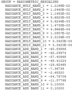
20: Calibration coefficients used to convert DN values to TOA radiance values for Landsat 8. By Anders Knudby, CC BY 4.0.
In order to produce a raster data layer in which each cell value is a measure of TOA radiance, you can therefore use the ‘Raster Calculator’ available in all GIS / remote sensing software, and some software packages even have dedicated ‘Landsat radiometric calibration’ tools that find the relevant information in the metadata and apply it for you.
Digital Numbers to TOA Reflectance
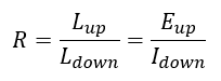
Converting DN values to a measure of radiance is an important step toward using remote sensing data in a quantitative way – in which the values in each cell have an actual physical meaning. However, there is one principal problem with radiance measurements: The radiance coming from an area depends both on the physical characteristics of that area, such as what is on the surface, but it also depends on the amount of radiation incident on that area. It is easy to confirm this with a single experiment: Move to a light switch near you, make sure it is on, and focus your gaze on a wall. Note how bright it is (a rough human approximation of the amount of radiance coming from it). Now turn off the light, and note whether the wall got darker or lighter. It got darker, of course, which means that there is now less radiance coming from it. And this happens although the wall itself did not change at all! In the remote sensing context, radiance measurements are therefore rarely used directly, but are typically used as a step toward a radiometric quantity that is more closely linked to the surface it is coming from: reflectance. For isotropic radiation, the reflectance (R) of a given area is the ratio of outgoing vs. incoming radiance, also often expressed on the basis of exitance (E) and irradiance (I):
In the wall example, when you turn off the light both the incoming and the outgoing radiance is reduced, and the reflectance of the wall is unchanged. That’s because the reflectance is a physical property of the wall that is independent of illumination. This makes it uniquely suitable for use in remote sensing, because multiple observations with varying illumination can be compared, for uses such as tracking change of an area through time, or for comparing different areas on Earth.
If we convert TOA radiance values to reflectance values, we get what’s called TOA reflectance, which is the reflectance of the entire Earth-Atmosphere system. To think about what that means, imagine that you are an astronaut and you put a hula-hoop ring horizontally right at the level of the top of the atmosphere (if the top of the atmosphere were possible to define and find!), and you then measure the amount of radiation passing through the ring in upward and downward directions. Dividing one by the other gives you TOA reflectance.
Calculating TOA reflectance is done a bit differently for different data types. For Landsat 8, there is another set of calibration coefficients that you can apply exactly like you can apply those for TOA radiance (Figure 21).
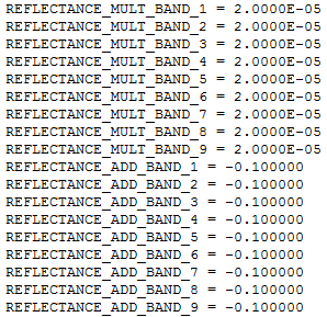
21: Calibration coefficients used to convert DN values to TOA reflectance values for Landsat 8. Note that values for bands 10 and 11 are not provided, because these bands do not measure reflected solar radiation (except to a negligible degree). Also note that coefficients are the same for all bands – for Landsat 8 the DN values have been specifically generated for each scene to ensure constant TOA reflectance calibration coefficients. By Anders Knudby, CC BY 4.0.
For older Landsat data, as well as for several other types of sensors, it is necessary to explicitly calculate the amount of incoming solar radiation at the top of the atmosphere, and divide the radiance by this value while correcting for the difference between radiance and irradiance and the angle of incoming solar radiation. This is done generically with the following equation (rearranged for pedagogical reasons from equation 4, page 79, in the Landsat 7 handbook), explained in more detail below:
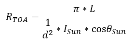
where RTOA is the top-of-atmosphere reflectance, L is (upward) radiance, d is the Earth-Sun distance in astronomical units, ISun is the mean extraterrestrial solar irradiance, and θSun is the solar zenith angle – the angle between the direction toward the Sun and the normal of the Earth’s surface. The equation is a division between the outgoing radiation in all upward directions (i.e. the exitance, in the numerator) and the incoming radiation in all downward directions (i.e. the irradiance, in the denominator).
The numerator is relatively simple: the upward radiance, L, which is quantified as the radiation per exposed unit surface area moving in directions within a specified solid angle, is multiplied by π to convert it to a value that quantifies radiation moving in all upward directions instead, to make it comparable to the incoming solar irradiance in the denominator.
In the denominator, we have ISun, the average incoming solar irradiance at the top of the atmosphere. Because the distance between the Sun and the Earth varies throughout the year and the amount of solar irradiance varies with it, we need to correct this by the factor 1/d2, where d is the actual distance between the Sun and the Earth when the image was acquired. If the Sun were at zenith (directly overhead), this would quantify the incoming irradiance per unit surface area. In cases when the Sun is not at zenith, we must multiply this value by the cosine of the solar zenith angle to arrive at the irradiance per exposed unit surface area.
Note: In the above two equations, the λ subscript indicating that these calculations must be performed on a band-by-band basis has been omitted for clarity, but keep this in mind. L varies by band, as does ISun, so both must be calculated specifically for each band to be correct.
With these calculations, you are able to convert the DN values in each pixel to a measure of TOA reflectance, which is a physical property of the Earth-Atmosphere system. This fact, that TOA reflectance is not an arbitrary number dependent on sensor calibration and illumination, but rather a physical property of the parts of the Earth seen in the image, allows us to use images captured by different sensors, at different times, and for different areas, and directly compare the values in each pixel. The one remaining problem in this approach is that most researchers are more interested in the reflectance of the Earth’s surface than in the reflectance at the top of the atmosphere, but the state of the atmosphere and the state of the surface both influence TOA reflectance. The next step to further process the data from each pixel is thus to remove the influence that the atmosphere has on these values, to arrive at a measure of surface reflectance!