9.5: Recasting the Shields Diagram
- Page ID
- 4208
\( \newcommand{\vecs}[1]{\overset { \scriptstyle \rightharpoonup} {\mathbf{#1}} } \)
\( \newcommand{\vecd}[1]{\overset{-\!-\!\rightharpoonup}{\vphantom{a}\smash {#1}}} \)
\( \newcommand{\id}{\mathrm{id}}\) \( \newcommand{\Span}{\mathrm{span}}\)
( \newcommand{\kernel}{\mathrm{null}\,}\) \( \newcommand{\range}{\mathrm{range}\,}\)
\( \newcommand{\RealPart}{\mathrm{Re}}\) \( \newcommand{\ImaginaryPart}{\mathrm{Im}}\)
\( \newcommand{\Argument}{\mathrm{Arg}}\) \( \newcommand{\norm}[1]{\| #1 \|}\)
\( \newcommand{\inner}[2]{\langle #1, #2 \rangle}\)
\( \newcommand{\Span}{\mathrm{span}}\)
\( \newcommand{\id}{\mathrm{id}}\)
\( \newcommand{\Span}{\mathrm{span}}\)
\( \newcommand{\kernel}{\mathrm{null}\,}\)
\( \newcommand{\range}{\mathrm{range}\,}\)
\( \newcommand{\RealPart}{\mathrm{Re}}\)
\( \newcommand{\ImaginaryPart}{\mathrm{Im}}\)
\( \newcommand{\Argument}{\mathrm{Arg}}\)
\( \newcommand{\norm}[1]{\| #1 \|}\)
\( \newcommand{\inner}[2]{\langle #1, #2 \rangle}\)
\( \newcommand{\Span}{\mathrm{span}}\) \( \newcommand{\AA}{\unicode[.8,0]{x212B}}\)
\( \newcommand{\vectorA}[1]{\vec{#1}} % arrow\)
\( \newcommand{\vectorAt}[1]{\vec{\text{#1}}} % arrow\)
\( \newcommand{\vectorB}[1]{\overset { \scriptstyle \rightharpoonup} {\mathbf{#1}} } \)
\( \newcommand{\vectorC}[1]{\textbf{#1}} \)
\( \newcommand{\vectorD}[1]{\overrightarrow{#1}} \)
\( \newcommand{\vectorDt}[1]{\overrightarrow{\text{#1}}} \)
\( \newcommand{\vectE}[1]{\overset{-\!-\!\rightharpoonup}{\vphantom{a}\smash{\mathbf {#1}}}} \)
\( \newcommand{\vecs}[1]{\overset { \scriptstyle \rightharpoonup} {\mathbf{#1}} } \)
\( \newcommand{\vecd}[1]{\overset{-\!-\!\rightharpoonup}{\vphantom{a}\smash {#1}}} \)
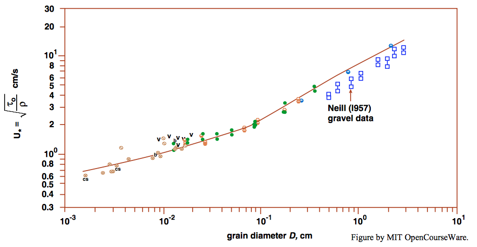
\(\newcommand{\avec}{\mathbf a}\) \(\newcommand{\bvec}{\mathbf b}\) \(\newcommand{\cvec}{\mathbf c}\) \(\newcommand{\dvec}{\mathbf d}\) \(\newcommand{\dtil}{\widetilde{\mathbf d}}\) \(\newcommand{\evec}{\mathbf e}\) \(\newcommand{\fvec}{\mathbf f}\) \(\newcommand{\nvec}{\mathbf n}\) \(\newcommand{\pvec}{\mathbf p}\) \(\newcommand{\qvec}{\mathbf q}\) \(\newcommand{\svec}{\mathbf s}\) \(\newcommand{\tvec}{\mathbf t}\) \(\newcommand{\uvec}{\mathbf u}\) \(\newcommand{\vvec}{\mathbf v}\) \(\newcommand{\wvec}{\mathbf w}\) \(\newcommand{\xvec}{\mathbf x}\) \(\newcommand{\yvec}{\mathbf y}\) \(\newcommand{\zvec}{\mathbf z}\) \(\newcommand{\rvec}{\mathbf r}\) \(\newcommand{\mvec}{\mathbf m}\) \(\newcommand{\zerovec}{\mathbf 0}\) \(\newcommand{\onevec}{\mathbf 1}\) \(\newcommand{\real}{\mathbb R}\) \(\newcommand{\twovec}[2]{\left[\begin{array}{r}#1 \\ #2 \end{array}\right]}\) \(\newcommand{\ctwovec}[2]{\left[\begin{array}{c}#1 \\ #2 \end{array}\right]}\) \(\newcommand{\threevec}[3]{\left[\begin{array}{r}#1 \\ #2 \\ #3 \end{array}\right]}\) \(\newcommand{\cthreevec}[3]{\left[\begin{array}{c}#1 \\ #2 \\ #3 \end{array}\right]}\) \(\newcommand{\fourvec}[4]{\left[\begin{array}{r}#1 \\ #2 \\ #3 \\ #4 \end{array}\right]}\) \(\newcommand{\cfourvec}[4]{\left[\begin{array}{c}#1 \\ #2 \\ #3 \\ #4 \end{array}\right]}\) \(\newcommand{\fivevec}[5]{\left[\begin{array}{r}#1 \\ #2 \\ #3 \\ #4 \\ #5 \\ \end{array}\right]}\) \(\newcommand{\cfivevec}[5]{\left[\begin{array}{c}#1 \\ #2 \\ #3 \\ #4 \\ #5 \\ \end{array}\right]}\) \(\newcommand{\mattwo}[4]{\left[\begin{array}{rr}#1 \amp #2 \\ #3 \amp #4 \\ \end{array}\right]}\) \(\newcommand{\laspan}[1]{\text{Span}\{#1\}}\) \(\newcommand{\bcal}{\cal B}\) \(\newcommand{\ccal}{\cal C}\) \(\newcommand{\scal}{\cal S}\) \(\newcommand{\wcal}{\cal W}\) \(\newcommand{\ecal}{\cal E}\) \(\newcommand{\coords}[2]{\left\{#1\right\}_{#2}}\) \(\newcommand{\gray}[1]{\color{gray}{#1}}\) \(\newcommand{\lgray}[1]{\color{lightgray}{#1}}\) \(\newcommand{\rank}{\operatorname{rank}}\) \(\newcommand{\row}{\text{Row}}\) \(\newcommand{\col}{\text{Col}}\) \(\renewcommand{\row}{\text{Row}}\) \(\newcommand{\nul}{\text{Nul}}\) \(\newcommand{\var}{\text{Var}}\) \(\newcommand{\corr}{\text{corr}}\) \(\newcommand{\len}[1]{\left|#1\right|}\) \(\newcommand{\bbar}{\overline{\bvec}}\) \(\newcommand{\bhat}{\widehat{\bvec}}\) \(\newcommand{\bperp}{\bvec^\perp}\) \(\newcommand{\xhat}{\widehat{\xvec}}\) \(\newcommand{\vhat}{\widehat{\vvec}}\) \(\newcommand{\uhat}{\widehat{\uvec}}\) \(\newcommand{\what}{\widehat{\wvec}}\) \(\newcommand{\Sighat}{\widehat{\Sigma}}\) \(\newcommand{\lt}{<}\) \(\newcommand{\gt}{>}\) \(\newcommand{\amp}{&}\) \(\definecolor{fillinmathshade}{gray}{0.9}\)The Shields diagram has a satisfying underlying physical significance, but it is awkward to use to find the threshold shear stress that corresponds to a given sediment diameter, or to find the largest sediment diameter that is moved by a given shear stress, because both \(\tau_{\text{o}}\) and \(D\) appear in both of the axis variables. (This exemplifies the difference between two contrasting goals, both of them laudatory but often in conflict: expressing results in a form that most directly reveals the underlying processes, or in a form that is most useful in practical work.) To get around this problem the Shields parameter and the boundary Reynolds number can easily be recast into two equivalent dimensionless variables, one with \(D\) but not \(\tau_{\text{o}}\) and the other with \(\tau_{\text{o}}\) but not \(D\). You can verify for yourself that these are \(\tau_{\text{o}}\left(\rho / \gamma^{\prime 2} \mu^{2}\right)^{1 / 3}\) and \(D\left(\rho \gamma^{\prime} / \mu^{2}\right)^{1 / 3}\). Figure \(\PageIndex{1}\) shows a recast version of the Shields diagram, From Miller et al. (1977). The axes in Figure \(\PageIndex{1}\) are labeled with \(u_{*}\) and \(D\), so the graph does not look dimensionless, but those values are for a water temperature of \(20^{\circ} \mathrm{C}\); the compilers just took the dimensionless graph, substituted in the \(20^{\circ}\) values of \(\rho\) and \(\mu\) into the axis variables, and ended up with the \(20^{\circ}\) values of \(u_{*}\) and \(D\). In effect, the graph is still really dimensionless.

One of the problems about the movement threshold is that there is a wide range of flow conditions for which there’s weak but noticeable sediment movement. That leads to the problem of how to define the condition of incipient movement in the first place. Quantitative criteria have been proposed, but they have not yet become firmly established. Nonetheless, the Shields diagram continues to be used, because it gives good ballpark results for both engineering and sedimentological purposes. Various investigators have tried to establish arbitrary but experimentally reproducible definitions of the beginning of movement.
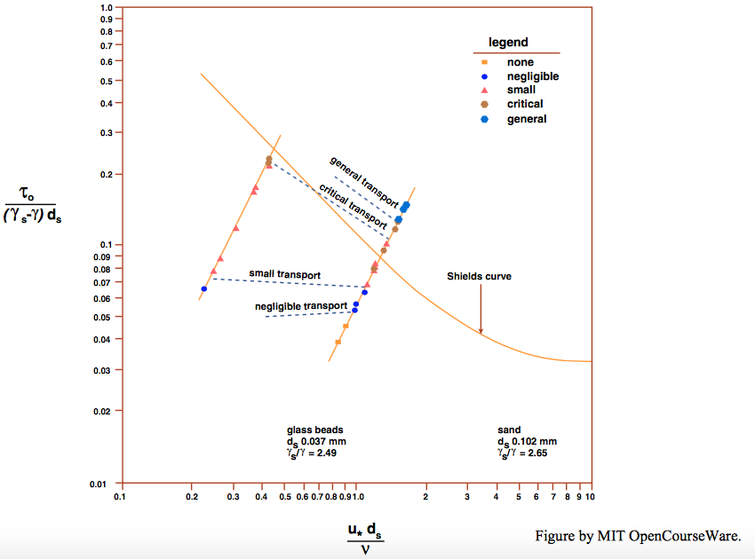
By observation of the bed through a microscope, Vanoni (1964) found that movement was intermittent on any small area of the bed, and, when it did occur, it took place in local gusts with several grains moving at once. He defined the critical stage of movement in terms of four gust frequencies (Figure \(\PageIndex{2}\)):
- negligible \((< 0.1\) \(\mathrm{s^{-1}}\))
- small (\(0.1–0.33\) \(\mathrm{s^{-1}}\))
- critical (\(0.33–1\) \(\mathrm{s^{-1}}\))
- general (\(>1\) \(\mathrm{s^{-1}}\))

Figure \(\PageIndex{2}\) makes clear how wide the range of condition is for which an objective observer, unschooled in the intricacies or defining incipient movement, might judge where to locate the threshold condition. As you have seen, this effect has even led some observers to question whether a criterion for inception of movement can even be formulated at all: movement tails off so gradually with decreasing flow strength that even in very weak flows, if one waits long enough one might see a particle moved by an instantaneous local fluid force on the bed, that is at the very extreme of the frequency distribution of such forces.
The Hjulström Diagram
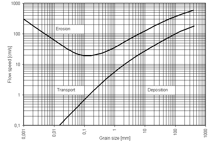
No account of the threshold of sediment movement would be complete without mention of the famous graph proposed long ago by Hjulström (1939) (reproduced without change here as Figure \(\PageIndex{3}\)), which has been used, or at least cited, by generations of sedimentationists. Hjulström undertook to represent the boundaries among erosion, transportation, and deposition in a graph of flow velocity vs. particle size. He acknowledged that use of the mean velocity to characterize the flow is inadequate, and viewed it as only “a temporary substitute until more data are available” (Hjulström, 1939, p. 9). The heavy bands between transportation and erosion, labeled “A”, were meant to represent the uncertainty of the data used to define the boundary. It is clear that Hjulström intended that band to represent the threshold of bed-load transport as the flow velocity is gradually increased. The word “erosion” in the graph is better read as “traction transport”: the former is best reserved for net removal of sediment from a given area of a sediment bed by the action of the fluid flow. (There can be transportation without erosion, if the sediment transport rate does not increase in the downstream direction and the local concentration of sediment in transport does not change with time.) The curve labeled “B” was meant to show cessation of transportation as the flow velocity gradually decreases; Hjulström relied upon some earlier flume observations that indicated that for sediments coarser than about medium sand the flow velocity for cessation of sediment movement about two-thirds that for inception of movement (see comments in the following paragraph). Hjulström showed the part of Curve B for fine sediments as a dashed line presumably because no data were available in that range. The widening gap between curves A and B is a consequence of the effect of cohesion increasing the velocities needed for initiation of movement. It seems likely that if the effects of cohesion in fine sediments could somehow be eliminated, the gap between curves A and B would be narrow for the entire range of sediment sizes.

The idea that the flow strength for cessation of movement is less than, rather than equal to, the flow strength for initiation of movement may have to do with a kind of hysteresis effect: as weak transport continues on a granular bed at about threshold conditions, the bed becomes partly armored, in the sense that most of the bed particles have found stable positions, and a small number of particles, not having found such positions and thus being the very most mobile, continue to pick their way across the immobile bed surface at flow strengths slightly lower than that for which inception of movement was judged to have begun. In any case, the range of flow velocities represented by the gap between Hjulström’s curves A and B lies within the rather wide range, noted in an earlier section, for which there is at least some weak transport, so the difference between the two curves seems not to be of great consequence.
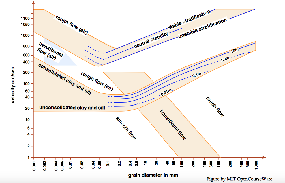
The Hjulström diagram was later modified by Sundborg (1956). Figure \(\PageIndex{4}\) shows Sundborg’s version, taken directly from the original. Sundborg’s graph shows separate curves for the movement threshold corresponding to several water depths, as is necessary if the flow velocity rather than the boundary shear stress (as in the Shields diagram) is used for the flow strength. The purpose of the lightly shaded band that includes these specific curves for the various flow velocities was not explicitly described, but it was probably meant to represent uncertainty in the data. Sundborg made note of Hjulström’s lower curve, for cessation of movement, but did not include it in his version.

Such are the origins of what might be called the Hjulström–Sundborg diagram. A diagram like Sundborg’s version, showing a family of threshold curves as a function of flow depth, with the curves based on the same data as the Shields diagram or its successors, has much potential for use by sedimentary geologists, despite the engineers’ aversion to using velocity rather than boundary shear stress for this purpose. Various versions of the Hjulström diagram have appeared in a great many textbooks and monographs since Sundborg’s contribution, but often in deplorably corrupted form: the curve for cessation of transportation is usually shown far lower than in the Hjulström original, with velocities lower than the curve for incipient movement by a factor of more than five!


