8.5: Variables
- Page ID
- 4202
\( \newcommand{\vecs}[1]{\overset { \scriptstyle \rightharpoonup} {\mathbf{#1}} } \)
\( \newcommand{\vecd}[1]{\overset{-\!-\!\rightharpoonup}{\vphantom{a}\smash {#1}}} \)
\( \newcommand{\id}{\mathrm{id}}\) \( \newcommand{\Span}{\mathrm{span}}\)
( \newcommand{\kernel}{\mathrm{null}\,}\) \( \newcommand{\range}{\mathrm{range}\,}\)
\( \newcommand{\RealPart}{\mathrm{Re}}\) \( \newcommand{\ImaginaryPart}{\mathrm{Im}}\)
\( \newcommand{\Argument}{\mathrm{Arg}}\) \( \newcommand{\norm}[1]{\| #1 \|}\)
\( \newcommand{\inner}[2]{\langle #1, #2 \rangle}\)
\( \newcommand{\Span}{\mathrm{span}}\)
\( \newcommand{\id}{\mathrm{id}}\)
\( \newcommand{\Span}{\mathrm{span}}\)
\( \newcommand{\kernel}{\mathrm{null}\,}\)
\( \newcommand{\range}{\mathrm{range}\,}\)
\( \newcommand{\RealPart}{\mathrm{Re}}\)
\( \newcommand{\ImaginaryPart}{\mathrm{Im}}\)
\( \newcommand{\Argument}{\mathrm{Arg}}\)
\( \newcommand{\norm}[1]{\| #1 \|}\)
\( \newcommand{\inner}[2]{\langle #1, #2 \rangle}\)
\( \newcommand{\Span}{\mathrm{span}}\) \( \newcommand{\AA}{\unicode[.8,0]{x212B}}\)
\( \newcommand{\vectorA}[1]{\vec{#1}} % arrow\)
\( \newcommand{\vectorAt}[1]{\vec{\text{#1}}} % arrow\)
\( \newcommand{\vectorB}[1]{\overset { \scriptstyle \rightharpoonup} {\mathbf{#1}} } \)
\( \newcommand{\vectorC}[1]{\textbf{#1}} \)
\( \newcommand{\vectorD}[1]{\overrightarrow{#1}} \)
\( \newcommand{\vectorDt}[1]{\overrightarrow{\text{#1}}} \)
\( \newcommand{\vectE}[1]{\overset{-\!-\!\rightharpoonup}{\vphantom{a}\smash{\mathbf {#1}}}} \)
\( \newcommand{\vecs}[1]{\overset { \scriptstyle \rightharpoonup} {\mathbf{#1}} } \)
\( \newcommand{\vecd}[1]{\overset{-\!-\!\rightharpoonup}{\vphantom{a}\smash {#1}}} \)
\(\newcommand{\avec}{\mathbf a}\) \(\newcommand{\bvec}{\mathbf b}\) \(\newcommand{\cvec}{\mathbf c}\) \(\newcommand{\dvec}{\mathbf d}\) \(\newcommand{\dtil}{\widetilde{\mathbf d}}\) \(\newcommand{\evec}{\mathbf e}\) \(\newcommand{\fvec}{\mathbf f}\) \(\newcommand{\nvec}{\mathbf n}\) \(\newcommand{\pvec}{\mathbf p}\) \(\newcommand{\qvec}{\mathbf q}\) \(\newcommand{\svec}{\mathbf s}\) \(\newcommand{\tvec}{\mathbf t}\) \(\newcommand{\uvec}{\mathbf u}\) \(\newcommand{\vvec}{\mathbf v}\) \(\newcommand{\wvec}{\mathbf w}\) \(\newcommand{\xvec}{\mathbf x}\) \(\newcommand{\yvec}{\mathbf y}\) \(\newcommand{\zvec}{\mathbf z}\) \(\newcommand{\rvec}{\mathbf r}\) \(\newcommand{\mvec}{\mathbf m}\) \(\newcommand{\zerovec}{\mathbf 0}\) \(\newcommand{\onevec}{\mathbf 1}\) \(\newcommand{\real}{\mathbb R}\) \(\newcommand{\twovec}[2]{\left[\begin{array}{r}#1 \\ #2 \end{array}\right]}\) \(\newcommand{\ctwovec}[2]{\left[\begin{array}{c}#1 \\ #2 \end{array}\right]}\) \(\newcommand{\threevec}[3]{\left[\begin{array}{r}#1 \\ #2 \\ #3 \end{array}\right]}\) \(\newcommand{\cthreevec}[3]{\left[\begin{array}{c}#1 \\ #2 \\ #3 \end{array}\right]}\) \(\newcommand{\fourvec}[4]{\left[\begin{array}{r}#1 \\ #2 \\ #3 \\ #4 \end{array}\right]}\) \(\newcommand{\cfourvec}[4]{\left[\begin{array}{c}#1 \\ #2 \\ #3 \\ #4 \end{array}\right]}\) \(\newcommand{\fivevec}[5]{\left[\begin{array}{r}#1 \\ #2 \\ #3 \\ #4 \\ #5 \\ \end{array}\right]}\) \(\newcommand{\cfivevec}[5]{\left[\begin{array}{c}#1 \\ #2 \\ #3 \\ #4 \\ #5 \\ \end{array}\right]}\) \(\newcommand{\mattwo}[4]{\left[\begin{array}{rr}#1 \amp #2 \\ #3 \amp #4 \\ \end{array}\right]}\) \(\newcommand{\laspan}[1]{\text{Span}\{#1\}}\) \(\newcommand{\bcal}{\cal B}\) \(\newcommand{\ccal}{\cal C}\) \(\newcommand{\scal}{\cal S}\) \(\newcommand{\wcal}{\cal W}\) \(\newcommand{\ecal}{\cal E}\) \(\newcommand{\coords}[2]{\left\{#1\right\}_{#2}}\) \(\newcommand{\gray}[1]{\color{gray}{#1}}\) \(\newcommand{\lgray}[1]{\color{lightgray}{#1}}\) \(\newcommand{\rank}{\operatorname{rank}}\) \(\newcommand{\row}{\text{Row}}\) \(\newcommand{\col}{\text{Col}}\) \(\renewcommand{\row}{\text{Row}}\) \(\newcommand{\nul}{\text{Nul}}\) \(\newcommand{\var}{\text{Var}}\) \(\newcommand{\corr}{\text{corr}}\) \(\newcommand{\len}[1]{\left|#1\right|}\) \(\newcommand{\bbar}{\overline{\bvec}}\) \(\newcommand{\bhat}{\widehat{\bvec}}\) \(\newcommand{\bperp}{\bvec^\perp}\) \(\newcommand{\xhat}{\widehat{\xvec}}\) \(\newcommand{\vhat}{\widehat{\vvec}}\) \(\newcommand{\uhat}{\widehat{\uvec}}\) \(\newcommand{\what}{\widehat{\wvec}}\) \(\newcommand{\Sighat}{\widehat{\Sigma}}\) \(\newcommand{\lt}{<}\) \(\newcommand{\gt}{>}\) \(\newcommand{\amp}{&}\) \(\definecolor{fillinmathshade}{gray}{0.9}\)It seems like a good idea at this point to think in a very general way about which variables are likely to be important in problems of sediment transport, and to organize those variables into a set of dimensionless variables that is likely to be useful as a framework from which to simplify or (complexify or specialize!) in any particular problem we deal with later. This is your chance to think about the phenomenon of sediment transport in its broadest aspects.
This endeavor involves some assumptions about what might be called the target flow. For the sake of definiteness, we will look at the movement of cohesionless sediment by steady uniform flows in straight rectangular channels of effectively infinite width in a nonrotating system. We thereby ignore the effects of channel width, cross-section shape, channel curvature, and the Earth’s rotation, and we restrict ourselves to equilibrium sediment transport. The first three restrictions are especially serious in fluvial sediment transport, but our target flow is a good start, from which these other effects can be evaluated. Ignoring the Earth’s rotation is not as serious as it might seem, because most aspects of sediment transport are tied up with the local near-bottom structure of turbulent shear flows, which, as you saw in Chapter 7, are about the same in geophysical flows as in actually or effectively nonrotating flows. Time-dependent problems in sediment transport are also of great importance, but again our target case represents a good reference. Finally, the assumption of cohesionless flows shuts us out of the complex, frustrating, and extremely important world of fine cohesive sediments—another topic that deserves its own separate set of notes.
The most important sediment-transport effects we will deal with in later chapters are easy to list:
- modes of grain movement
- speeds of grain movement
- sediment load
- sediment transport rate
- bed configuration
Variables
Which variables might have a role in influencing or determining these effects? The possibilities form a long list (and there probably are others I have not thought of):
Sediment:
- joint size–shape–density distribution
- elastic properties
Fluid:
- density \(\rho\)
- viscosity \(\mu\)
- specific weight (weight per unit volume) \(\gamma\)
- elastic properties
- thermal properties
- surface tension
Flow:
- mean depth \(d\)
- mean velocity \(U\)
- discharge (per unit width) \(q\)
- boundary shear stress \(\tau_{\text{o}}\)
- slope \(S\)
- power \(P\)
System:
- acceleration of gravity \(g\)
Clearly this list is too long: some items can safely be neglected, and some items are actually redundant.
First, here are some comments on the variables that characterize the sediment. There are no redundancies in the items for the sediment in the above list, but they are effectively non-quantifiable because of grain shape. And even if grain shape is neglected, the size–density distribution has to be characterized by a two-variable joint frequency distribution (see Figure 8.1.3). As mentioned earlier, a good approximation in practice might be to assume one dominant blade-shaped spike in the distribution corresponding to crudely quartz-density sediment, and one or more subsidiary spikes for heavy minerals (Figure 8.1.4). It is common practice in work on sediment transport to assume that all grains have the same density, so that the sediment can be characterized by the mean or median size \(D\) and the density \(\rho_{s}\). Adding the standard deviation \(\sigma\) of the size distribution makes for three variables describing the sediment.
With regard to variables characterizing the flow, there is a serious redundancy in the foregoing list: only two variables are needed to specify the bulk flow, one of them being the flow depth and the other a flow-strength variable. The two most logical candidates for the flow-strength variable are the boundary shear stress \(\tau_{\text{o}}\) and the mean velocity \(U\) (or the surface velocity \(U_{s}\)). (Some might take exception to that statement, however, and claim that the flow power \(P\) is the most fundamental flow-strength variable.)
In choosing the flow-strength variable, we could address three considerations:
- Which variables specify or characterize the state of sediment transport, in the sense that specification of those variables unambiguously corresponds to or identifies the state of sediment movement, whether those variables are imposed upon the system or are themselves fixed by the operation of the system?
- Which variables are truly independent, in the sense that they are imposed on the system and are unaffected by its operation?
- Which variables govern the state of sediment transport, in the sense that they are dynamically most directly responsible for particle transport and bed- configuration development, whether or not they are independent?
One of the important goals in studying the phenomena of sediment transport is to show as clearly and unambiguously as possible the hydraulic relationships among those phenomena. It would be good to have a one-to-one correlation between sediment-transport states and combinations of variables, because that would represent the clearest start on knowing what we have to deal with or explain.
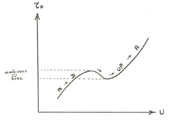
In terms of unambiguous characterization, \(U\) and \(d\) (or \(q\) and \(d\)) are the most appropriate variables to describe the flow because, for a given fluid, for each combination of \(U\) and \(d\) in steady uniform flow there is one and only one average state of the flow, in terms of velocity structure and boundary forces. This is not the case, however, if \(\tau_{\text{o}}\) or \(P\) is used in place of \(U\) or \(q\): if \(\tau_{\text{o}}\) or \(P\) is used, there is an element of ambiguity in that for certain variables values of \(\tau_{\text{o}}\) or \(P\) more than one bed state at a given flow depth is possible. Although I am getting ahead of myself in bringing up this matter before the chapter on bed configurations, I will point out here that this has to do with the substantial decrease in form resistance in the transition from ripples or dunes to plane bed with increasing \(U\) or \(q\) at constant \(d\). You can see from the cartoon graph in Figure \(\PageIndex{1}\) that because of this effect there is a non-negligible range of \(\tau_{\text{o}}\) for which three different values of \(U\) are possible. But you can see from the graph that if you specify \(U\), you thereby uniquely specify \(\tau_{\text{o}}\). An alternative approach would be to use only the part of \(\tau_{\text{o}}\), called the skin friction, that represents the local shear forces on the bed, and leave out of consideration the part of \(\tau_{\text{o}}\), called the form drag, that arises from large-scale pressure differences on the fore and aft sides of roughness elements. The ambiguity noted above would thereby be circumvented. The problem is that although there are several published procedures for such a drag partition, none works remarkably well (yet).

Independence need not be a criterion in choice of variables to describe the state of sediment transport, because a given set of variables can equally well describe the state of sediment transport whether any given variable in the set is dependent or independent: the state of sediment transport is a function of the nature of the flow but not of how the flow is arranged or established, provided that the flow is strong enough at the outset to produce general sediment movement on the bed.
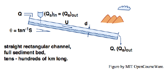
Independence of variables depends to a great extent upon the nature of the sediment-transporting system. For an example of this, think about an extremely long channel (tens of kilometers, say) with bottom slope \(S\), straight vertical sidewalls, and an erodible sediment bed, into which a constant water discharge \(Q\) is introduced at the upstream end (Figure \(\PageIndex{2}\)). Assume that after a transient period of flow adjustment a steady state is maintained by introducing sediment at the upstream end at a rate equal to the sediment discharge \(Q_{s}\) at the downstream end. The imposed variables here are \(Q\) and \(S\); \(Q_{s}\), \(U\), and \(d\) are adjusted by the flow. Because of the great channel length, flow and sediment transport are virtually uniform along most of the channel except near the upstream and downstream ends. Even though the flow might prefer a different \(S\) for the given \(Q\), adjustment in \(S\) is so slow that, on time scales that are short in terms of geologic time but long in terms of bed-form movement, \(S\) can be considered fixed. Hence \(Q\) and \(S\) are independent variables, and \(U\) and \(d\) along with all variables that express the details of flow structure and sediment transport are dependent upon \(Q\) and \(S\).

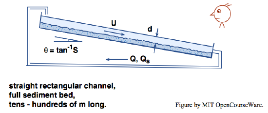
In a similar but much shorter channel, tens of meters, say (Figure \(\PageInded{3}\)), \(S\) can change so rapidly by erosion and deposition along the channel that the flow cannot be considered uniform until \(S\) has reached a state of adjustment to the imposed \(Q\); \(Q\) is an independent variable, but \(S\) is now dependent, in the sense that it cannot be preset except approximately by manipulation of \(d\) by means of a gate or weir at an overfall at the downstream end of the channel. And in constant-volume recirculating channels, in which there is no overfall, \(d\) is truly independent and \(S\) is truly dependent.

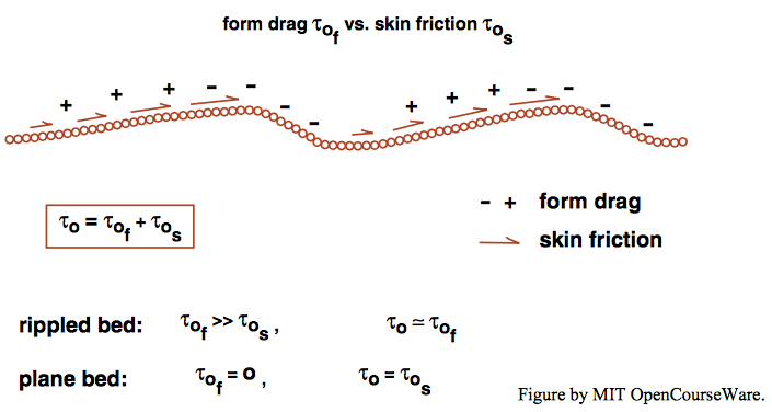
With regard to governing variables, at first thought \(\tau_{\text{o}}\) is a more logical choice than \(U\) for characterizing the effect of the flow on the bed, because the force exerted by the flow on the bed is what causes the sediment transport in the first place. And for transport over planar bed surfaces, that is certainly true. But you will see in a later chapter that, over a wide range of flow and sediment conditions, the flow molds the bed into rugged flow-transverse ridges called bed forms. On beds covered with such bed forms, only a small part of \(\tau_{\text{o}}\) represents the boundary friction that is directly responsible for grain transport, the rest being form drag on the main roughness elements (Figure \(\PageIndex{4}\)). In such situations, therefore, \(\tau_{\text{o}}\) is as much a surrogate variable as \(U\), in the sense that it is not directly responsible for particle transport and bed-form development, as are near-bed flow structure and distribution of boundary skin friction in space and time. These latter, however, are themselves uniquely characterized by \(U\) and \(d\).

When bed forms are present, the spatially and temporally averaged local skin friction would seem to be a better variable than \(\tau_{\text{o}}\) in characterizing the state of sediment transport, because it is free from the ambiguity mentioned above but at the same time is more directly responsible for the sediment movement. The trouble is that it cannot be measured, and it can be estimated only with considerable uncertainty using presently available drag-partition approaches.
Several variables on the list are of minor or negligible importance in most sediment-transport problems: the elastic and thermal properties of the fluid and the sediment, and the surface tension of the fluid.
So the final minimal list of variables that describe sediment transport in our target flow is as follows:
- Mean flow velocity \(U\) or boundary shear stress \(\tau_{\text{o}}\)
- Mean flow depth \(d\)
- Fluid density \(\rho\)
- Fluid viscosity \(\mu\)
- Median sediment diameter \(D\)
- Sediment sorting \(\sigma\)
- Sediment density \(\rho_{s}\)
- Acceleration of gravity \(g\) or submerged sediment specific weight \(\gamma^{\prime}\)
There are eight variables on the list, so we should expect to have an equivalent set of five dimensionless variables that describe the state of sediment transport equally well. A great many different sets are possible: you can choose a variety of sets of three repeating variables, and then you could manipulate those sets further by multiplying and dividing the various individual dimensionless variables in those sets.
In general, we could move in one (or both) of two directions at this point. We could try to develop a set that has the greatest relevance to the physical effects involved in the sediment transport, or we could try to develop a set that has the sedimentologically most relevant or interesting variables segregated into different dimensionless variables.
With regard to sets of dimensionless variables that are relevant to the physical effects of sediment transport, I will mention just two possibilities:
| \(\frac{\tau_{o}}{\gamma^{\prime} D}\) | Shields parameter, a dimensionless \(\tau_{\text{o}}\) |
| \(\frac{\rho u_{*} D}{\mu}\) | roughness Reynolds number, \(\text{Re}_{*}\) |
| \(d/D\) | relative roughness |
| \(\frac{\rho_{s}}{\rho}\) | density ratio |
| \(\frac{\sigma}{D}\) | sorting-to-size ratio |
You could construct this set by using \(\tau_{\text{o}}\), \(\rho\), and \(D\) as repeaters. The physical significance of the roughness Reynolds number was discussed back in Chapter 4. The Shields parameter also has a clear physical significance. The fluid force on bed particles is approximately proportional to \(\tau_{\text{o}}D^{2}\), whereas the weight of the bed particles is proportional to \(\gamma^{\prime}D^{3}\). The ratio of these two quantities is the Shields parameter, so the Shields parameter is proportional to the ratio of the fluid force on particles to the weight of the particles. For that reason it could also be called a mobility number.
Another dynamically meaningful set of dimensionless variables can be formed using U as the flow-strength variable:
| \(\frac{\rho U d}{\mu}\) |
Reynolds number based on depth and velocity |
| \(\frac{U}{(g d)^{1 / 2}}\) |
Froude number based on depth and velocity |
| \(d/D\) | relative roughness |
| \(\frac{\rho_{s}}{\rho}\) | density ratio |
| \(\frac{\sigma}{D}\) | sorting-to-size ratio |
The repeaters in this set are \(\rho\), \(U\), and \(d\). The mean-flow Reynolds number describes the structure of the mean flow, and the mean-flow Froude number is relevant to the energy state of the flow, as discussed in Chapter 5.
Probably the most useful set of dimensionless variables for the purpose of unambiguous description of the state of flow and sediment transport is one in which the sedimentologically interesting variables \(U\), \(d\), and \(D\) are segregated into separate dimensionless variables:
| \(\left(\frac{\rho \gamma^{\prime}}{\mu^{2}}\right)^{1 / 3} d\) |
dimensionless flow depth \(d^{\text{o}}\) |
| \(\left(\frac{\rho^{2}}{\mu \gamma^{\prime}}\right)^{1 / 3} U\) |
dimensionless flow velocity \(U^{\text{o}}\) |
| \(\left(\frac{\rho \gamma^{\prime}}{\mu^{2}}\right)^{1 / 3} D\) |
dimensionless sediment size \(D^{\text{o}}\) |
| \(\frac{\rho_{s}}{\rho}\) | density ratio |
| \(\frac{\sigma}{D}\) | sorting-to-size ratio |
The repeaters for this set are \(\rho\), \(\mu\), and \(\gamma^{\prime}\).


