
9.5.1: Escoffier's model
- Page ID
- 16405

\( \newcommand{\vecs}[1]{\overset { \scriptstyle \rightharpoonup} {\mathbf{#1}} } \)
\( \newcommand{\vecd}[1]{\overset{-\!-\!\rightharpoonup}{\vphantom{a}\smash {#1}}} \)
\( \newcommand{\id}{\mathrm{id}}\) \( \newcommand{\Span}{\mathrm{span}}\)
( \newcommand{\kernel}{\mathrm{null}\,}\) \( \newcommand{\range}{\mathrm{range}\,}\)
\( \newcommand{\RealPart}{\mathrm{Re}}\) \( \newcommand{\ImaginaryPart}{\mathrm{Im}}\)
\( \newcommand{\Argument}{\mathrm{Arg}}\) \( \newcommand{\norm}[1]{\| #1 \|}\)
\( \newcommand{\inner}[2]{\langle #1, #2 \rangle}\)
\( \newcommand{\Span}{\mathrm{span}}\)
\( \newcommand{\id}{\mathrm{id}}\)
\( \newcommand{\Span}{\mathrm{span}}\)
\( \newcommand{\kernel}{\mathrm{null}\,}\)
\( \newcommand{\range}{\mathrm{range}\,}\)
\( \newcommand{\RealPart}{\mathrm{Re}}\)
\( \newcommand{\ImaginaryPart}{\mathrm{Im}}\)
\( \newcommand{\Argument}{\mathrm{Arg}}\)
\( \newcommand{\norm}[1]{\| #1 \|}\)
\( \newcommand{\inner}[2]{\langle #1, #2 \rangle}\)
\( \newcommand{\Span}{\mathrm{span}}\) \( \newcommand{\AA}{\unicode[.8,0]{x212B}}\)
\( \newcommand{\vectorA}[1]{\vec{#1}} % arrow\)
\( \newcommand{\vectorAt}[1]{\vec{\text{#1}}} % arrow\)
\( \newcommand{\vectorB}[1]{\overset { \scriptstyle \rightharpoonup} {\mathbf{#1}} } \)
\( \newcommand{\vectorC}[1]{\textbf{#1}} \)
\( \newcommand{\vectorD}[1]{\overrightarrow{#1}} \)
\( \newcommand{\vectorDt}[1]{\overrightarrow{\text{#1}}} \)
\( \newcommand{\vectE}[1]{\overset{-\!-\!\rightharpoonup}{\vphantom{a}\smash{\mathbf {#1}}}} \)
\( \newcommand{\vecs}[1]{\overset { \scriptstyle \rightharpoonup} {\mathbf{#1}} } \)
\( \newcommand{\vecd}[1]{\overset{-\!-\!\rightharpoonup}{\vphantom{a}\smash {#1}}} \)
\(\newcommand{\avec}{\mathbf a}\) \(\newcommand{\bvec}{\mathbf b}\) \(\newcommand{\cvec}{\mathbf c}\) \(\newcommand{\dvec}{\mathbf d}\) \(\newcommand{\dtil}{\widetilde{\mathbf d}}\) \(\newcommand{\evec}{\mathbf e}\) \(\newcommand{\fvec}{\mathbf f}\) \(\newcommand{\nvec}{\mathbf n}\) \(\newcommand{\pvec}{\mathbf p}\) \(\newcommand{\qvec}{\mathbf q}\) \(\newcommand{\svec}{\mathbf s}\) \(\newcommand{\tvec}{\mathbf t}\) \(\newcommand{\uvec}{\mathbf u}\) \(\newcommand{\vvec}{\mathbf v}\) \(\newcommand{\wvec}{\mathbf w}\) \(\newcommand{\xvec}{\mathbf x}\) \(\newcommand{\yvec}{\mathbf y}\) \(\newcommand{\zvec}{\mathbf z}\) \(\newcommand{\rvec}{\mathbf r}\) \(\newcommand{\mvec}{\mathbf m}\) \(\newcommand{\zerovec}{\mathbf 0}\) \(\newcommand{\onevec}{\mathbf 1}\) \(\newcommand{\real}{\mathbb R}\) \(\newcommand{\twovec}[2]{\left[\begin{array}{r}#1 \\ #2 \end{array}\right]}\) \(\newcommand{\ctwovec}[2]{\left[\begin{array}{c}#1 \\ #2 \end{array}\right]}\) \(\newcommand{\threevec}[3]{\left[\begin{array}{r}#1 \\ #2 \\ #3 \end{array}\right]}\) \(\newcommand{\cthreevec}[3]{\left[\begin{array}{c}#1 \\ #2 \\ #3 \end{array}\right]}\) \(\newcommand{\fourvec}[4]{\left[\begin{array}{r}#1 \\ #2 \\ #3 \\ #4 \end{array}\right]}\) \(\newcommand{\cfourvec}[4]{\left[\begin{array}{c}#1 \\ #2 \\ #3 \\ #4 \end{array}\right]}\) \(\newcommand{\fivevec}[5]{\left[\begin{array}{r}#1 \\ #2 \\ #3 \\ #4 \\ #5 \\ \end{array}\right]}\) \(\newcommand{\cfivevec}[5]{\left[\begin{array}{c}#1 \\ #2 \\ #3 \\ #4 \\ #5 \\ \end{array}\right]}\) \(\newcommand{\mattwo}[4]{\left[\begin{array}{rr}#1 \amp #2 \\ #3 \amp #4 \\ \end{array}\right]}\) \(\newcommand{\laspan}[1]{\text{Span}\{#1\}}\) \(\newcommand{\bcal}{\cal B}\) \(\newcommand{\ccal}{\cal C}\) \(\newcommand{\scal}{\cal S}\) \(\newcommand{\wcal}{\cal W}\) \(\newcommand{\ecal}{\cal E}\) \(\newcommand{\coords}[2]{\left\{#1\right\}_{#2}}\) \(\newcommand{\gray}[1]{\color{gray}{#1}}\) \(\newcommand{\lgray}[1]{\color{lightgray}{#1}}\) \(\newcommand{\rank}{\operatorname{rank}}\) \(\newcommand{\row}{\text{Row}}\) \(\newcommand{\col}{\text{Col}}\) \(\renewcommand{\row}{\text{Row}}\) \(\newcommand{\nul}{\text{Nul}}\) \(\newcommand{\var}{\text{Var}}\) \(\newcommand{\corr}{\text{corr}}\) \(\newcommand{\len}[1]{\left|#1\right|}\) \(\newcommand{\bbar}{\overline{\bvec}}\) \(\newcommand{\bhat}{\widehat{\bvec}}\) \(\newcommand{\bperp}{\bvec^\perp}\) \(\newcommand{\xhat}{\widehat{\xvec}}\) \(\newcommand{\vhat}{\widehat{\vvec}}\) \(\newcommand{\uhat}{\widehat{\uvec}}\) \(\newcommand{\what}{\widehat{\wvec}}\) \(\newcommand{\Sighat}{\widehat{\Sigma}}\) \(\newcommand{\lt}{<}\) \(\newcommand{\gt}{>}\) \(\newcommand{\amp}{&}\) \(\definecolor{fillinmathshade}{gray}{0.9}\)A tidal inlet is not fixed but a dynamic entity governed by important factors such as tidal currents, storms, the tidal prism (the storage volume of the estuary between low tide and high tide level) and littoral sediment transport. Escoffier (1940) was the first to study the stability of the cross-sectional area of the inlet proper. Because of the littoral drift leaving and entering the inlet with the tide, there can be a considerable variation of the cross-sectional area.
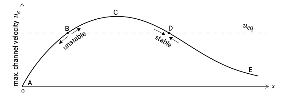
Escoffier’s predominantly qualitative study led to an expression for the maximum cross-sectionally averaged entrance channel velocity (\(u_e\), with the subscript indicating the entrance) for a given estuary or inlet (see Intermezzo 9.4 for an approximation). He related \(u_e\) to the hydraulic radius of the channel (\(R\)), its cross-sectional area (\(A_e\)) and the tidal range in the estuary (\(\Delta h\)). Since this calculation is made for a given inlet, other variables such as the channel bed roughness, its length, the surface area of the inlet, and the tidal range at sea have then all become more or less constant. Escoffier combined the variables for a given inlet into a single parameter, \(x\), such that a larger entrance cross-section results in a larger value of \(x\). Qualitatively, he found that \(u_e\) varied as a function of \(x\) more or less as shown in Fig. 9.22.
The maximum cross-sectional velocity is the maximum velocity during the tidal cycle. To understand its behaviour as a function of the cross-sectional area, it can be approximated as the amplitude \(\hat{u}_e\) of a sinusoidal tidal motion \(u\). In that case we can relate the maximum cross-sectionally averaged entrance velocity \(u_e = \hat{u}_e\) to the tidal prism \(P\). The tidal prism \(P\) is equal to the time integral of the inflow during flood or to the outflow during ebb (cf. Eq. 9.2.3.1):
\[P = \int_{0}^{1/2T} A_e u dt = \int_{0}^{1/2T} A_e \hat{u}_e \sin \left (\dfrac{2\pi}{T} t \right ) dt = \dfrac{TA_e}{\pi} \hat{u}_e\]
and thus:
\[\hat{u}_e = \dfrac{\pi P}{A_e T} \label{eq9.5.1.2}\]
with \(T\) being the tidal period.
A curve like in Fig. 9.22 is called a closure curve. In the range from \(A\) to \(C\) on this curve, the entrance channel is so small that it chokes off the tidal flow so that the tidal difference within the estuary will be less than at sea. For that reason the channel velocity will increase for an increasing cross-section. In terms of Eq. \(\ref{eq9.5.1.2}\): with increasing \(A_e\), \(P\) increases so much that \(\hat{u}_e\) increases. On section C-E of the curve, the tidal flow is not choked off any longer (now \(P\) remains constant for increasing \(A\)) such that the maximum current velocity decreases as the channel becomes larger. For an arbitrary estuary or inlet, a closure curve can be computed using a hydrodynamic model. This can be either a numerical model or a simpler analytical model. Simplified analytical solutions can for instance be obtained by assuming a short basin that responds in pumping mode (a uniformly fluctuating water level, see Sect. 5.7.3).
Escoffier’s next step was to introduce the concept of an equilibrium maximum velocity \(u_{eq}\), below which the velocity in the channel is too low to erode sediment and keep the entrance channel open. This critical velocity is more or less independent of the channel geometry, according to Escoffier, and he plotted it as a horizontal line on Fig. 9.22, viz. independent of the cross-section. In reality \(u_{eq}\) is generally a weak function of the cross-sectional area, but at first order this effect can be neglected.
The fate of an estuary or tidal inlet can now be predicted by examining the curve ACE in relation to \(u_{eq}\). Obviously, if \(u_e\) is always less than \(u_{eq}\) (for all values of \(x\) the closure curve lies below \(u_{eq}\)) then any sediment deposited in the entrance will remain there and the estuary will be closed off eventually. However, if a curve of \(u_e\) versus \(x\) intersects the \(u_{eq}\) line as shown at B and D in Fig. 9.22, then a variety of situations can exist. If for example, the channel dimensions place it on section A-B of the curve in Fig. 9.22, then the channel is too small and the friction too high to maintain itself; so it will be closed by natural processes. If the channel geometry places it on section D-E of the curve, it will also become smaller, but as it does so, the velocity, ue, will increase; sedimentation continues until point D is reached. Lastly, if the channel configuration places it on section B-D of the curve, then erosion takes place until point D is again reached; point D represents a stable situation. Since \(u_e = u_{eq}\) represents the stable (D) and unstable (B) equilibrium conditions, the relationship for \(u_{eq}\) is called the equilibrium flow curve or the stability curve. The equilibrium velocity curve that Escoffier introduced assumes that the equilibrium velocity, \(u_{eq}\), is a constant that depends only on the sediment diameter, and suggests that a good approximation of the velocity is 3 ft/s (0.9 m/s).
With this insight, it is now possible to evaluate the influence of changes in an estuary mouth. Since point D represents a naturally stable situation, most natural estuaries will tend to lie more or less in that region. Of course, a severe storm can cause severe sedimentation, largely filling the entrance, which is then suddenly in the state represented by section A–B of the curve. In such a situation, immediate dredging is called for to prevent complete closure. It is not necessary to restore the original situation, however, since once the entrance geometry places it on section B–C–D of the curve in the figure, nature will do the rest of the work given enough time. Apparently, Escoffier’s model incorporates a feedback between hydrodynamics and morphology and can therefore be seen as a morphodynamic model for the entrance of tidal basin.
Shipping interests may make it desirable to enlarge the entrance of a given estuary to accommodate larger ships. If such an expansion scheme places the channel on section D–E of the curve, the dredging industry will remain profitable for the foreseeable future. It may be possible to carry out the expansion and still prevent continual dredging by changing the channel alignment and artificially constricting its width – techniques often used in rivers – so that the larger channel cross-section remains stable. Translating such changes into a figure such as Fig. 9.22 means that a new curve of \(u_{e}\) versus \(x\) has been generated which generally yields a slightly higher value of \(u_{e}\) for a given \(x\) value. This results in point D, the equilibrium situation, being moved to the right in the figure.