3.4.3: Spectral Analysis

An alternative way of arriving at a statistical representation of the sea state uses the fact that the surface elevation at one location can be unraveled into various sine waves with different frequencies of which the amplitudes and phases can be determined by so-called Fourier analysis. Fourier demonstrated that any signal can be described by a sum of harmonic components, a so-called Fourier series. Under the assumption of a stationary record these sine waves have a constant amplitude and phase per component in time. For a time-record with finite duration the Fourier series can be written in terms of sine (or cosine) functions that fit an integer number of times in the record duration \(T_r\).

The oscillatory surface elevation can be written as a Fourier series as follows:

\[\eta = \sum_{n = 1}^{N} a_n \cos (2\pi f_n t + \alpha_n)\label{eq3.4.3.1}\]

where

\[f_n = \dfrac{n}{T_r} \text{ for } n = 1, 2, ... \nonumber\]

Although in nature the frequencies will be continuous, the frequencies in Eq. \(\ref{eq3.4.3.1}\) are discrete by necessity because in practice the length of the wave series is restricted to for instance 20 min (\(\Delta f = 1/T_r\)). The record length thus determines the smallest frequency (the longest wave) that can be determined from the record: \(f_{\min} = 1/T_r\). Moreover the time series is not continuous since the water level measurements are performed with a certain sampling interval. The sampling interval determines the highest frequency that can be determined from the record: \(f_{\max} = \tfrac{1}{2\Delta t}\).

From the amplitudes of the various components the spectrum of wave energy over the range of wave periods or frequencies can be calculated. With a bit of trigonometry it can be found that for one harmonic component the variance is equal to \(\tfrac{1}{2} a_n^2\). Then for a sum of harmonic components the corresponding variance is given by:

\[\sum_{n = 1}^{N} \dfrac{1}{2} a_n^2\]

The variance density spectrum gives the variance density per unit frequency interval for each frequency and is constant for \(\Delta f \to 0\):

\[\lim_{\Delta f \to 0} \dfrac{1/2a_n^2}{\Delta f} = E(f_n) \label{eq3.4.3.3}\]

By taking the integral of the spectrum the total variance is recovered again:

\[\int_{0}^{\infty} E(f) df = \overline{\eta^2} = \sigma^2 \label{eq3.4.3.4}\]

Two conclusions can be drawn. First, in the spectrum the variance density is the contribution of one component to the total variance. Second, the standard deviation \(\sigma\) of the surface elevation signal can be estimated from the area under the spectrum. Note further that from the variance density spectrum the energy density spectrum is readily obtained, since variance and energy are coupled through Eq. 3.4.2.1.

The so-computed spectrum describes the time-series under consideration but is only an estimation of the spectrum representing the random process, since a next realisation under the same condition will give a slightly different surface elevation. To get a better estimate averaging has to take place of spectra based on subdivisions of the time series or equivalently over frequency bins.

Figure 3.7: Surface elevation time series and corresponding spectra for sea and swell combined (upper panel), sea (middle panel) and swell (lower panel). To generate the sea component a so-called JONSWAP spectrum (a typical spectrum for sea, see Sect. 3.5.1) is used with \(H_S= 1.8 m\), \(T_p = 5.5s\) and a peak enhancement factor \(\gamma = 1\). For the swell component, \(H_S = 0.5m\) \(T_p = 12s\) and \(\gamma = 5\) are used. For both sea and swell the peak-width parameter is \(\sigma = 0.07\) for \(f \le f_p\) and \(\sigma = 0.09\) for \(f > f_p\). The sea and swell spectra are combined in a bi-modal spectrum of swell and sea. The timeseries are generated from the spectra at a sampling frequency of 25 Hz assuming random phases. Note that the timeseries in the right panels correspond to Fig. 3.6.

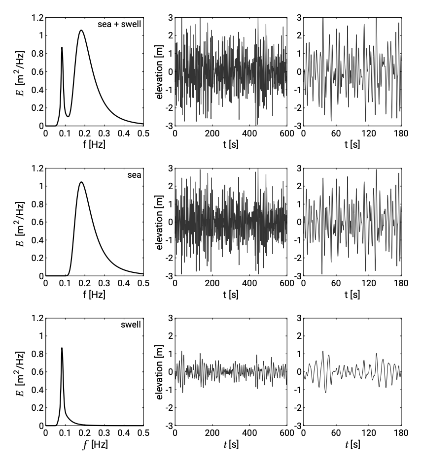
In Fig. 3.7 energy spectra are shown with the corresponding time series. In the middle and lower panel all energy is concentrated around the mid-frequencies. The narrower the spectrum the more regular the waves are. For larger, longer waves the spectrum will be shifted towards the lower frequencies and contain more energy. For smaller, shorter waves the spectrum will be shifted towards the higher frequencies and be lower. Sometimes one can distinguish between two adjacent or often partly overlapping parts of the spectrum. This means that two distinct wave fields are present: swell and sea (upper panel). If the mean frequencies of the two wave fields are close then there will be so much overlap that the spectrum is broad but otherwise looks like a spectrum with only one wave field.

What about the phases of the different components? The distribution of the phases over the frequencies is called a phase spectrum. Often the phase spectrum is not shown since in not too steep waves and in deep water the phases seem to be independent of each other and uniformly distributed between \(-\pi\) and \(\pi\). This means that the different components are not related through the phases and can be seen as individual waves moving independently through the signal as if they were alone. This is the case for linear small amplitude waves. So then only the amplitude or variance/energy spectrum remains to characterise the wave record.

Which parameters can be derived from the variance spectrum? First, the spectrum reveals the dominant frequencies in the wave record; most energy occurs at the spectral peak and the corresponding wave period is called the peak spectral period \(T_p\). Other characteristic average parameters can be expressed in terms of spectral moments:

\[m_n = \int_{0}^{\infty} f^n E(f) df \ \ \text{ for }\ n = ..., -3, -2, -1, 0, 1, 2, 3, ...\]

\(m_0\) is the area under the spectrum. Since \(m_0\) is the total variance integrated over all frequencies, the standard deviation is given by \(\sigma = \sqrt{m_0}\) (see Eqs. \(\ref{eq3.4.3.3}\) and \(\ref{eq3.4.3.4}\)). In Sect. 3.4.4 we will see how the zero-th moment \(m_0\) and the second moment can be used to determine the zero-crossing period from the spectrum.