12.2: The Final Project

The final project will test your ability to make an observation of the atmosphere and to provide an integrated analysis of that observation using the knowledge and quantitative analysis skills that you have learned in this course.

Final Project 1

1. Choose an observation of the atmosphere. The observation could be a picture, video, radar image, satellite image, or figure. It can come from you, the course material, a site that allows copying, or a family member or friend. Do not use an observation that has been previously analyzed by anyone else. When you are choosing an observation, think about the story you want to tell and how well you think you can tell it. You will want to do a little research and maybe think about two or three different possibilities before you settle on one.
2. Check to make sure that your observation is at a time and place for which you can get weather information (e.g., temperature, relative humidity, pressure, weather maps, weather station model, upper air data) that you will need to analyze and explain your observation.
3. Before you start the analysis and writing, send me an email with your observation and a few words about it so that I can approve it. I must approve your choice of an observation.
4. Gather the evidence as you build your analysis of the observation. Be sure to document where your evidence came from.
5. First show and describe the observation. You should give as much information as you have about the observation – what, where, and when it was observed.
6. Write your analysis in formal language, such as you might see in a science news magazine and is in the example below. You can submit this analysis as a Word or pdf file. The length could be as short as a few pages, including figures, graphs, and equations, but it must be thorough and complete.
7. Be thorough but concise.
8. After you have completed your final project, go back through it and edit it. Make it as polished and appealing as possible.
9. Follow the instructions below for submitting it in Canvas. Late presentations will have points deducted.
   1. Put your final project in either Word or PDF format.
   2. Embed pictures and equations in the text.
   3. Name your file "Final_Project_YourLastName".
   4. Submit it to the Final Project assignment which is located in the Lesson 12 Module in Canvas.
10. Follow the instructions below for submitting it in Canvas.

Final Project 2

1. Choose an observation of the atmosphere. The observation could be a picture, video, radar image, satellite image, or figure. It can come from you, the course material, a site that allows copying, or a family member or friend. Do not use an observation that has been previously analyzed by anyone else. When you are choosing an observation, think about the story you want to tell and how well you think you can tell it. You will want to do a little research and maybe think about two or three different possibilities before you settle on one. Try to think of observations that are unique and interesting.
2. Check to make sure that your observation is at a time and place for which you can get weather information (e.g., temperature, relative humidity, pressure, weather maps, weather station model, upper air data) that you will need to analyze and explain your observation.
3. Before you start the analysis and writing, send me an email with your observation and a few words about it so that I can approve it. I must approve your choice of an observation.
4. Gather the evidence as you build your analysis of the observation. Be sure to document where your evidence came from.
5. First show and describe the observation. You should give as much information as you have about the observation—what, where, and when it was observed.
6. Then make a 5-minute PowerPoint presentation of your observation and your analysis. The length could be as short as a few slides, including figures, graphs, and equations, but it must be thorough and complete. I suggest that you use anywhere from three to about six slides, depending on the number of figures you need to describe your analysis. Put in another slide with your references to websites, books, and papers on it. You do not have to do a quantitative analysis, necessarily, but if you do, your analysis will be more impressive and convincing.
7. Be thorough but concise.
8. After you have completed your final project, go back through it and edit it. Make it as polished and appealing as possible.
9. Follow the instructions below for submitting it in Canvas. Late presentations will have points deducted.
   1. Put your final project in either PowewrPoint or PDF format.
   2. Embed pictures and equations in the text.
   3. Name your file "Final_Project_YourLastName".
   4. Submit it to the Final Project assignment which is located in the Lesson 12 Module in Canvas.
10. Presentations will run for two weeks. I will select the order of the presentations using random numbers, so you will need to attend all the classes. I will also take role during each class and will deduct participation points for students who do not have a valid excuse approved by me to miss class. It is only fair to the students who are presenting near the end that the audience is as big for the last presentation as it is for the first.

Example of a Final Project

Observation

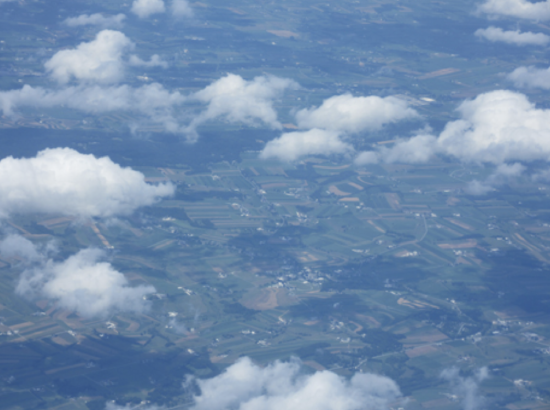
I took this picture of southeastern Pennsylvania while flying to Atlanta, GA on 29 June 2015. The picture was taken at 14:30 EDT (18:30 UTC) from an altitude of about 20 kft. Note the fair weather cumulus clouds have little vertical development. Also, even though it was a fairly moist summer day, the boundary layer below the fair weather cumulus appears quite clear.

Explanation

The presence of clouds indicates that three conditions existed: moisture, aerosol, and cooling. The moisture came from the surface, which had seen heavy rain a day before. Surface heating by solar visible irradiance evaporated liquid water on the surface, which created pockets of moist, buoyant air. These air parcels rose relative to the nearby less buoyant environment, according to the Buoyancy Equation [2.66]:

\[B=\frac{\left(T_{v}^{\prime}-T_{v}\right)}{T_{v}} g\]

until they reached the lifting condensation level (LCL). There, they became supersaturated, so that the aerosol that forms the cloud condensation nuclei nucleated and cloud drops were formed according to the Koehler Theory Equation [5.13]:

\[s_{k}=S_{k}-1=\frac{a_{K}}{r_{d}}-\frac{B i N_{s}}{r_{d}}\]

These clouds sat in the entrainment zone just above the convective boundary layer. The energy budget for such a recently wetted land surface would likely show significant downward net radiation, and significant upward latent heat flux.

The clouds showed little vertical development. This behavior would suggest that the air was quite stable. Indeed, the radiosonde recording (Figure 1) from Dulles Airport a few hours earlier indicated that the air was quite stable, with the ascent on a moist adiabat from the Lifting Condensation Level 5–10 K below the ambient temperature.

Figure 1. Skew-T from nearby Dulles International Airport on 29 June 2015.

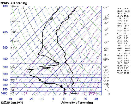
Credit: NWS data, University of Wyoming skew-T website

This condition came about from the synoptic scale conditions, with high pressure over the region (Figure 2) suggesting downward vertical descent and divergence according to Equation [9.5]:

\[\frac{\partial w}{\partial z}=-\vec{\nabla}_{H} \bullet \vec{U}_{H}\]

which, by adiabatic compression, would lead to clearing skies.

Figure 2. Surface weather map for 29 June 2015. Note the surface high pressure region over northern Virginia.

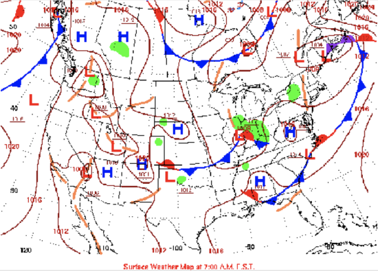
Credit: NOAA

It is most likely that these clouds in the observation were formed by adiabatic ascent by random localized buoyant air parcels. However, there was a fairly uniform stratus deck just to the northeast of this location and some evidence that this air mass was moving to the west or southwest toward the location (Figure 3).

Figure 3. Visible satellite image for 29 June 2015. Note the breaking cloud cover in the Northeast and the fair weather cumulus over much of Pennsylvania and Maryland.

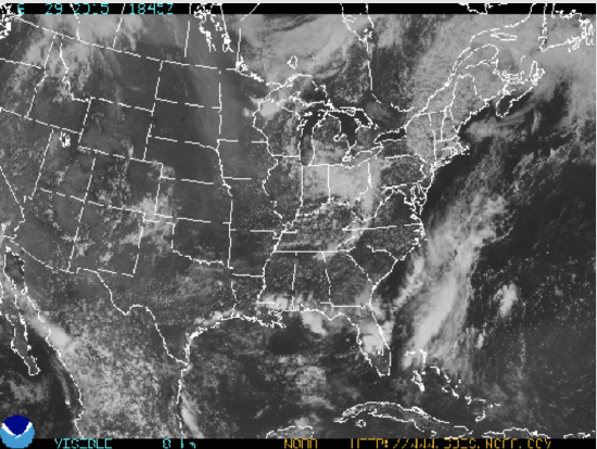
Credit: NOAA

As this stratus deck was mixed with drier air (Lesson 5.3, Equation [5.4]), the cloud deck could have broken up into evaporating individual clouds. Likely the clouds in the observation were from both adiabatic ascent and the evaporation of the stratus cloud deck.

Often with clear skies the pollution levels are high and the boundary layer is filled with haze. However, the visibility is quite good in the picture. There is generally enough PM2.5 (particle matter less than 2.5 microns in diameter) present in southeastern Pennsylvania. However, rain the previous day was able to remove some of the pollution from previous days, thus clearing the air. In addition, the particles that were there may not have been swollen to a size that efficiently scatters solar radiation, when in Equation [6.17]:

\[x \equiv \frac{2 \pi r}{\lambda}\]

the size of the particles are approximately equal to the visible wavelength. Indeed, we have at least three pieces of evidence that the air was fairly dry (Figure 1, Figure 3, and Figure 4 (Lesson 7)), with dewpoints in the middle-to-high 50s (^oF) (see this image).

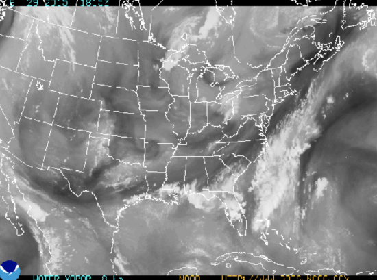
Figure 4. Satellite water vapor image for 29 June 2015. Note the tongue of fairly dry air going across western Virginia into Maryland and southeastern Pennsylvania.

Credit: NOAA

From the skew-T, the relative humidity was only about 50% (Lesson 3.5, RH = w/w_s = 7 g/kg / 14 g/kg). Thus, the recent scavenging of aerosol by heavy rain and the low relative humidity made for great visibility and clear boundary layer air even in the high pressure region, with light winds and clearing skies. This example is interesting because only after frontal passages with rain is the boundary layer air so clear under high pressure. If the high pressure were to persist, then the moisture levels would likely increase due to evaporation of surface water and the pollutant emissions and chemistry would make more particle pollution, both of which would lead to lower visibility in the boundary layer.

_________________________________

Self Evaluation of This Example. Note: This evaluation is given here to show you how the rubic will be used to evaluate your project. You should not include a self-evaluation with your project.

This example meets the overall standards for integration and explanation of the observation. The analysis addresses the presence of the fair weather cumulus and the reason for the clear air in conditions when the visibility is often not so good. On the other hand, my example would not receive a perfect score for a few reasons. First, the choice of observation is good but not very interesting. Second, all of the equations are appropriate, but some are not well integrated into the analysis. Third, some of the figures are fuzzy. And, fourth, the possible evaporation of the stratus deck is not particularly well explained.

For your reference, the grade for this example would likely be 11 to 12 on a scale of 15.

Final Project

(15% of final grade)

1. The final project is worth 15% of your final grade.
2. I will use the following rubric to grade your final project:

Final Project Grading Rubric

Evaluation	Explanation	Available % Points
Not Completed	Student did not complete the assignment by the due date.	0
Student completed the project with little attention to detail or effort.	Project is on a weak observation, has flawed analysis, and/or lacks a clear presentation. In addition, there is inadequate evidence of integration of course material, no references to equations that would help quantify the observation, or no/poor figures to support analysis.	3
Student completed the project, but it has many inadequacies.	Project is strong in one or two of the following areas but weak in the rest: good choice of observation, thorough analysis and evidence, conclusions supported by evidence, draws evidence from at least five different lessons, includes at least three different equations needed to do a quantitative analysis, contains figures/graphs taken from other sources to provide evidence and support conclusions, organization is logical, and presentation is clear and concise.	6
Student completed a pretty good project, but it had some inadequacies.	Project is strong in more than half of the following areas but weak in the rest: good choice of observation, thorough analysis and evidence, conclusions supported by evidence, draws evidence from at least five different lessons, includes at least three different equations needed to do a quantitative analysis, contains figures/graphs taken from other sources to provide evidence and support conclusions, organization is logical, and presentation is clear and concise.	9
Student completed a very good project, but it had a few inadequacies.	Project is strong in all but a few of the following areas: good choice of observation, thorough analysis and evidence, conclusions supported by evidence, draws evidence from at least five different lessons, includes at least three different equations needed to do a quantitative analysis, contains figures/graphs taken from other sources to provide evidence and support conclusions, organization is logical, and presentation is clear and concise.	12
Project is strong in all but a few of the following areas: good choice of observation, thorough analysis and evidence, conclusions supported by evidence, draws evidence from at least five different lessons, includes at least three different equations needed to do a quantitative analysis, contains figures/graphs taken from other sources to provide evidence and support conclusions, organization is logical, and presentation is clear and concise.	Project is strong in all of the following areas: good choice of observation, thorough analysis and evidence, conclusions supported by evidence, draws evidence from at least five different lessons, includes at least three different equations needed to do a quantitative analysis, contains figures/graphs taken from other sources to provide evidence and support conclusions, organization is logical, and	15