11.9: How Kinematic Fluxes Move Air Vertically
- Page ID
- 3423
\( \newcommand{\vecs}[1]{\overset { \scriptstyle \rightharpoonup} {\mathbf{#1}} } \)
\( \newcommand{\vecd}[1]{\overset{-\!-\!\rightharpoonup}{\vphantom{a}\smash {#1}}} \)
\( \newcommand{\id}{\mathrm{id}}\) \( \newcommand{\Span}{\mathrm{span}}\)
( \newcommand{\kernel}{\mathrm{null}\,}\) \( \newcommand{\range}{\mathrm{range}\,}\)
\( \newcommand{\RealPart}{\mathrm{Re}}\) \( \newcommand{\ImaginaryPart}{\mathrm{Im}}\)
\( \newcommand{\Argument}{\mathrm{Arg}}\) \( \newcommand{\norm}[1]{\| #1 \|}\)
\( \newcommand{\inner}[2]{\langle #1, #2 \rangle}\)
\( \newcommand{\Span}{\mathrm{span}}\)
\( \newcommand{\id}{\mathrm{id}}\)
\( \newcommand{\Span}{\mathrm{span}}\)
\( \newcommand{\kernel}{\mathrm{null}\,}\)
\( \newcommand{\range}{\mathrm{range}\,}\)
\( \newcommand{\RealPart}{\mathrm{Re}}\)
\( \newcommand{\ImaginaryPart}{\mathrm{Im}}\)
\( \newcommand{\Argument}{\mathrm{Arg}}\)
\( \newcommand{\norm}[1]{\| #1 \|}\)
\( \newcommand{\inner}[2]{\langle #1, #2 \rangle}\)
\( \newcommand{\Span}{\mathrm{span}}\) \( \newcommand{\AA}{\unicode[.8,0]{x212B}}\)
\( \newcommand{\vectorA}[1]{\vec{#1}} % arrow\)
\( \newcommand{\vectorAt}[1]{\vec{\text{#1}}} % arrow\)
\( \newcommand{\vectorB}[1]{\overset { \scriptstyle \rightharpoonup} {\mathbf{#1}} } \)
\( \newcommand{\vectorC}[1]{\textbf{#1}} \)
\( \newcommand{\vectorD}[1]{\overrightarrow{#1}} \)
\( \newcommand{\vectorDt}[1]{\overrightarrow{\text{#1}}} \)
\( \newcommand{\vectE}[1]{\overset{-\!-\!\rightharpoonup}{\vphantom{a}\smash{\mathbf {#1}}}} \)
\( \newcommand{\vecs}[1]{\overset { \scriptstyle \rightharpoonup} {\mathbf{#1}} } \)
\( \newcommand{\vecd}[1]{\overset{-\!-\!\rightharpoonup}{\vphantom{a}\smash {#1}}} \)
\(\newcommand{\avec}{\mathbf a}\) \(\newcommand{\bvec}{\mathbf b}\) \(\newcommand{\cvec}{\mathbf c}\) \(\newcommand{\dvec}{\mathbf d}\) \(\newcommand{\dtil}{\widetilde{\mathbf d}}\) \(\newcommand{\evec}{\mathbf e}\) \(\newcommand{\fvec}{\mathbf f}\) \(\newcommand{\nvec}{\mathbf n}\) \(\newcommand{\pvec}{\mathbf p}\) \(\newcommand{\qvec}{\mathbf q}\) \(\newcommand{\svec}{\mathbf s}\) \(\newcommand{\tvec}{\mathbf t}\) \(\newcommand{\uvec}{\mathbf u}\) \(\newcommand{\vvec}{\mathbf v}\) \(\newcommand{\wvec}{\mathbf w}\) \(\newcommand{\xvec}{\mathbf x}\) \(\newcommand{\yvec}{\mathbf y}\) \(\newcommand{\zvec}{\mathbf z}\) \(\newcommand{\rvec}{\mathbf r}\) \(\newcommand{\mvec}{\mathbf m}\) \(\newcommand{\zerovec}{\mathbf 0}\) \(\newcommand{\onevec}{\mathbf 1}\) \(\newcommand{\real}{\mathbb R}\) \(\newcommand{\twovec}[2]{\left[\begin{array}{r}#1 \\ #2 \end{array}\right]}\) \(\newcommand{\ctwovec}[2]{\left[\begin{array}{c}#1 \\ #2 \end{array}\right]}\) \(\newcommand{\threevec}[3]{\left[\begin{array}{r}#1 \\ #2 \\ #3 \end{array}\right]}\) \(\newcommand{\cthreevec}[3]{\left[\begin{array}{c}#1 \\ #2 \\ #3 \end{array}\right]}\) \(\newcommand{\fourvec}[4]{\left[\begin{array}{r}#1 \\ #2 \\ #3 \\ #4 \end{array}\right]}\) \(\newcommand{\cfourvec}[4]{\left[\begin{array}{c}#1 \\ #2 \\ #3 \\ #4 \end{array}\right]}\) \(\newcommand{\fivevec}[5]{\left[\begin{array}{r}#1 \\ #2 \\ #3 \\ #4 \\ #5 \\ \end{array}\right]}\) \(\newcommand{\cfivevec}[5]{\left[\begin{array}{c}#1 \\ #2 \\ #3 \\ #4 \\ #5 \\ \end{array}\right]}\) \(\newcommand{\mattwo}[4]{\left[\begin{array}{rr}#1 \amp #2 \\ #3 \amp #4 \\ \end{array}\right]}\) \(\newcommand{\laspan}[1]{\text{Span}\{#1\}}\) \(\newcommand{\bcal}{\cal B}\) \(\newcommand{\ccal}{\cal C}\) \(\newcommand{\scal}{\cal S}\) \(\newcommand{\wcal}{\cal W}\) \(\newcommand{\ecal}{\cal E}\) \(\newcommand{\coords}[2]{\left\{#1\right\}_{#2}}\) \(\newcommand{\gray}[1]{\color{gray}{#1}}\) \(\newcommand{\lgray}[1]{\color{lightgray}{#1}}\) \(\newcommand{\rank}{\operatorname{rank}}\) \(\newcommand{\row}{\text{Row}}\) \(\newcommand{\col}{\text{Col}}\) \(\renewcommand{\row}{\text{Row}}\) \(\newcommand{\nul}{\text{Nul}}\) \(\newcommand{\var}{\text{Var}}\) \(\newcommand{\corr}{\text{corr}}\) \(\newcommand{\len}[1]{\left|#1\right|}\) \(\newcommand{\bbar}{\overline{\bvec}}\) \(\newcommand{\bhat}{\widehat{\bvec}}\) \(\newcommand{\bperp}{\bvec^\perp}\) \(\newcommand{\xhat}{\widehat{\xvec}}\) \(\newcommand{\vhat}{\widehat{\vvec}}\) \(\newcommand{\uhat}{\widehat{\uvec}}\) \(\newcommand{\what}{\widehat{\wvec}}\) \(\newcommand{\Sighat}{\widehat{\Sigma}}\) \(\newcommand{\lt}{<}\) \(\newcommand{\gt}{>}\) \(\newcommand{\amp}{&}\) \(\definecolor{fillinmathshade}{gray}{0.9}\)Now that we know how to separate out the mean and turbulent parts, we can look at the concept of kinematic flux. A flux is the transfer of some variable per unit area per unit time. Generally in meteorology, we care about variables like mass, heat (i.e., temperature), kinetic energy, moisture, momentum. Those who study the atmosphere's composition are also interested in the flux of chemicals emitted into the atmosphere from the surface and the flux of atmospheric pollutants, such as ozone, back to Earth's surface. For this discussion, let's consider only the fluxes directly relevant to meteorology.
So the Sl units of the following fluxes would be \(\mathrm{kg} \mathrm{m}^{-2} \mathrm{s}^{-1}\) for mass \((m)\) \(\mathrm{kg}_{\text {water }} \mathrm{m}^{-2} \mathrm{s}^{-1}\) for moisture \(\left(m_{y}\right) ;\left(\mathrm{kg}\, \mathrm{m} \mathrm{s}^{-1}\right) \mathrm{m}^{-2} \mathrm{s}^{-1}=\mathrm{kg} \,\mathrm{m}^{-1} \mathrm{s}^{-2}\) for momentum \((m v),\) and \(\mathrm{J} \mathrm{m}^{-2} \mathrm{s}^{-1}\) for heat \(\left(m c_{p} T_{v}\right)\) or \(\mathrm{W} \mathrm{m}^{-2}\) (just like radiation).
We can write these in the kinematic form by dividing by the density of air:
- kinematic mass \(\mathrm{flux}=\left(\mathrm{kg}\, \mathrm{m}^{-2}\, \mathrm{s}^{-1}\right) /\left(\mathrm{kg} \,\mathrm{m}^{-3}\right)=\mathrm{m} \mathrm{s}^{-1}\)
- kinematic moisture \(\mathrm{flux}=\left(\mathrm{kg}_{\text {water }} \mathrm{m}^{-2} \mathrm{s}^{-1}\right) /\left(\mathrm{kg}_{\text {air }} \mathrm{m}^{-3}\right)=\mathrm{kg}_{\text {water }} \mathrm{kg}_{\text {air }}^{-1} \mathrm{ms}^{-1}\)
- kinematic momentum \(\mathrm{flux}=\mathrm{kg} \mathrm{m}^{-1} \mathrm{s}^{-2} /\left(\mathrm{kg} \mathrm{m}^{-3}\right)=\mathrm{m}^{2} \mathrm{s}^{-2}\)
For kinematic heat flux, the heat flux is usually divided by the air density times the specific heat of air to give units of \(\left(\mathbf{J} \mathbf{m}^{-2} \mathbf{s}^{-1}\right) /\left(\mathbf{k} \mathbf{g} \mathbf{m}^{-3} \mathbf{J} \mathbf{k} \mathbf{g}^{-1} \mathbf{K}^{-1}\right)=\mathbf{K} \mathbf{m} \mathbf{s}^{-1} .\) Note that this is just a temperature times a velocity.
The word “kinematic” is often dropped and assumed.
Let’s look at the kinematic heat flux in the vertical direction. Also, we are interested in the vertical transport of thermal energy and so we do not want to think about the adiabatic variation in temperature due to vertical motion, since an air parcel's temperature decreases with height even in adiabatic ascent. We can accomplish this by using the potential temperature and not the virtual temperature, which falls off with height adiabatically while the potential temperature is constant with height. θ does not equal T except at 1000 hPa, so we need to keep that in mind.
Write down the expression for the vertical flux of potential temperature, which is just equal to the vertical wind times the potential temperature, and then take the Reynolds average of that flux:
\[\overline{w \theta}=\bar{w} \bar{\theta}+\overline{w^{\prime} \theta^{\prime}}\]
The first term on the right is the vertical flux of potential temperature due to the average vertical motion, but w ~ 0 on average in the boundary layer, so we can usually drop the first term on the right.
Let’s consider how this flux works at moving thermal energy. A typical condition for the mixed boundary layer is a superadiabatic layer near the heated surface (i.e., θ decreases with height).

Let’s look at the different cases.
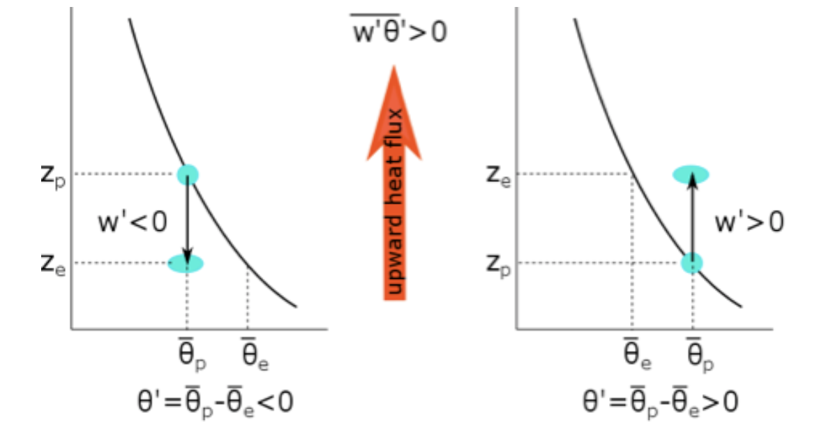
Daytime case with surface heating such that\(\partial \theta / \partial z<0\)(as in figure above). Eddies can make air trade places. They move some air parcels down,
for \[w^{\prime}<0\] and \[\theta^{\prime}<0: \overline{w^{\prime} \theta^{\prime}}>0\]
and at the same time move some up,
for \[w^{\prime}>0\] and \[\theta^{\prime}>0: \quad \overline{w^{\prime} \theta^{\prime}}>0\]
Both of these processes are happening simultaneously. If the air parcels mix at their new heights, they move cooler air lower (left panel above) or warmer air higher (right panel above) and in both cases, they move heat up. Thus, when the potential temperature decreases with height (i.e., is superadiabatic), the turbulent eddies move warmer air up and the heat flux is positive.

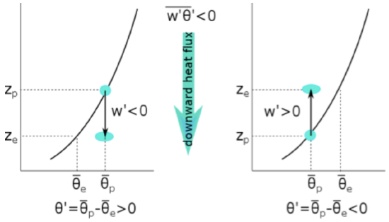
Nighttime case with surface cooling such that ∂θ/∂z > 0∂θ/∂z > 0 (see figure above). Eddies make air parcels trade places vertically. They move some air parcels down,
for \[w^{\prime}<0\] and \[\theta^{\prime}>0: \overline{w^{\prime} \theta^{\prime}}<0\]
and some up,
for \[w^{\prime}>0\] and \[\theta^{\prime}<0: \quad \overline{w^{\prime} \theta^{\prime}}<0\]
Both of these processes are happening simultaneously. If the air parcels mix at their new heights, they either move warmer air lower (left panel above) or cooler air higher (right panel above), and in both cases, they move heat down. Thus, when the potential temperature increases with height (i.e., is subadiabatic), the turbulent eddies move warmer air down and the heat flux is negative.
We see that by turbulent motions, the thermal energy tends to flow from higher mean temperature to lower mean temperature, or to put it another way, down the gradient of the mean value.
So, the heat flux \(\overline{w^{\prime} \theta^{\prime}}\) tells us about the transport of thermal energy by eddies.
Note that the transport is in the direction from the higher values to the lower values for the mean potential temperature. The heat flux is the way that sensible heat gets transferred to the free troposphere in the atmosphere's energy budget. The heat flux combined with the moisture flux create conditions that can lead to thunderstorms and severe weather.
Watch the following video (1:49) for further discussion of the eddy heat flux:
Eddy Heat Flux
- Click here for transcript of the Eddy Heat Flux.
-
Eddy fluxes are one of the most important concepts in the planetary boundary layer because they are responsible for most of the vertical transport of everything in the planetary boundary layer, both those things leaving the surface, and those things coming back down to Earth. In the horizontal, the mean winds do most of the transporting. But in the vertical, the eddies do most of the transporting. Let's look at the transport of potential temperature, which is the same as the transport of thermal energy, or heat. Consider first a super eddy body potential temperature profile, that is one in which the potential temperature decreases with height. We get these kinds of profiles on hot, sunny days. Usually eddies cycle some air down and other air up. An air parcel cycled up is warmer than the surrounding air, so the perturbation to the potential temperature, which is just the difference between the potential temperature of the parcel minus the potential temperature of the surrounding air, is positive. The perturbation to the vertical wind is also positive, since the air parcel is being brought up. So that the product of w prime and theta prime is positive. The eddy also moves colder air down into warmer surroundings. So the negative perturbation to the vertical wind brings a negative perturbation to the potential temperature, and the product that these two perturbations-- two negatives-- is positive. Taking these two parts of the eddy together, we see that the cold air has replaced warm air at the lower height, and warmer air has replaced colder air at the greater height, and thus the eddy flux is upward. Convince yourself that the drawing in figure 11.6 all give downward heat flux.


