8.4: Describing weather requires coordinate systems.
- Page ID
- 3399
\( \newcommand{\vecs}[1]{\overset { \scriptstyle \rightharpoonup} {\mathbf{#1}} } \)
\( \newcommand{\vecd}[1]{\overset{-\!-\!\rightharpoonup}{\vphantom{a}\smash {#1}}} \)
\( \newcommand{\id}{\mathrm{id}}\) \( \newcommand{\Span}{\mathrm{span}}\)
( \newcommand{\kernel}{\mathrm{null}\,}\) \( \newcommand{\range}{\mathrm{range}\,}\)
\( \newcommand{\RealPart}{\mathrm{Re}}\) \( \newcommand{\ImaginaryPart}{\mathrm{Im}}\)
\( \newcommand{\Argument}{\mathrm{Arg}}\) \( \newcommand{\norm}[1]{\| #1 \|}\)
\( \newcommand{\inner}[2]{\langle #1, #2 \rangle}\)
\( \newcommand{\Span}{\mathrm{span}}\)
\( \newcommand{\id}{\mathrm{id}}\)
\( \newcommand{\Span}{\mathrm{span}}\)
\( \newcommand{\kernel}{\mathrm{null}\,}\)
\( \newcommand{\range}{\mathrm{range}\,}\)
\( \newcommand{\RealPart}{\mathrm{Re}}\)
\( \newcommand{\ImaginaryPart}{\mathrm{Im}}\)
\( \newcommand{\Argument}{\mathrm{Arg}}\)
\( \newcommand{\norm}[1]{\| #1 \|}\)
\( \newcommand{\inner}[2]{\langle #1, #2 \rangle}\)
\( \newcommand{\Span}{\mathrm{span}}\) \( \newcommand{\AA}{\unicode[.8,0]{x212B}}\)
\( \newcommand{\vectorA}[1]{\vec{#1}} % arrow\)
\( \newcommand{\vectorAt}[1]{\vec{\text{#1}}} % arrow\)
\( \newcommand{\vectorB}[1]{\overset { \scriptstyle \rightharpoonup} {\mathbf{#1}} } \)
\( \newcommand{\vectorC}[1]{\textbf{#1}} \)
\( \newcommand{\vectorD}[1]{\overrightarrow{#1}} \)
\( \newcommand{\vectorDt}[1]{\overrightarrow{\text{#1}}} \)
\( \newcommand{\vectE}[1]{\overset{-\!-\!\rightharpoonup}{\vphantom{a}\smash{\mathbf {#1}}}} \)
\( \newcommand{\vecs}[1]{\overset { \scriptstyle \rightharpoonup} {\mathbf{#1}} } \)
\( \newcommand{\vecd}[1]{\overset{-\!-\!\rightharpoonup}{\vphantom{a}\smash {#1}}} \)
\(\newcommand{\avec}{\mathbf a}\) \(\newcommand{\bvec}{\mathbf b}\) \(\newcommand{\cvec}{\mathbf c}\) \(\newcommand{\dvec}{\mathbf d}\) \(\newcommand{\dtil}{\widetilde{\mathbf d}}\) \(\newcommand{\evec}{\mathbf e}\) \(\newcommand{\fvec}{\mathbf f}\) \(\newcommand{\nvec}{\mathbf n}\) \(\newcommand{\pvec}{\mathbf p}\) \(\newcommand{\qvec}{\mathbf q}\) \(\newcommand{\svec}{\mathbf s}\) \(\newcommand{\tvec}{\mathbf t}\) \(\newcommand{\uvec}{\mathbf u}\) \(\newcommand{\vvec}{\mathbf v}\) \(\newcommand{\wvec}{\mathbf w}\) \(\newcommand{\xvec}{\mathbf x}\) \(\newcommand{\yvec}{\mathbf y}\) \(\newcommand{\zvec}{\mathbf z}\) \(\newcommand{\rvec}{\mathbf r}\) \(\newcommand{\mvec}{\mathbf m}\) \(\newcommand{\zerovec}{\mathbf 0}\) \(\newcommand{\onevec}{\mathbf 1}\) \(\newcommand{\real}{\mathbb R}\) \(\newcommand{\twovec}[2]{\left[\begin{array}{r}#1 \\ #2 \end{array}\right]}\) \(\newcommand{\ctwovec}[2]{\left[\begin{array}{c}#1 \\ #2 \end{array}\right]}\) \(\newcommand{\threevec}[3]{\left[\begin{array}{r}#1 \\ #2 \\ #3 \end{array}\right]}\) \(\newcommand{\cthreevec}[3]{\left[\begin{array}{c}#1 \\ #2 \\ #3 \end{array}\right]}\) \(\newcommand{\fourvec}[4]{\left[\begin{array}{r}#1 \\ #2 \\ #3 \\ #4 \end{array}\right]}\) \(\newcommand{\cfourvec}[4]{\left[\begin{array}{c}#1 \\ #2 \\ #3 \\ #4 \end{array}\right]}\) \(\newcommand{\fivevec}[5]{\left[\begin{array}{r}#1 \\ #2 \\ #3 \\ #4 \\ #5 \\ \end{array}\right]}\) \(\newcommand{\cfivevec}[5]{\left[\begin{array}{c}#1 \\ #2 \\ #3 \\ #4 \\ #5 \\ \end{array}\right]}\) \(\newcommand{\mattwo}[4]{\left[\begin{array}{rr}#1 \amp #2 \\ #3 \amp #4 \\ \end{array}\right]}\) \(\newcommand{\laspan}[1]{\text{Span}\{#1\}}\) \(\newcommand{\bcal}{\cal B}\) \(\newcommand{\ccal}{\cal C}\) \(\newcommand{\scal}{\cal S}\) \(\newcommand{\wcal}{\cal W}\) \(\newcommand{\ecal}{\cal E}\) \(\newcommand{\coords}[2]{\left\{#1\right\}_{#2}}\) \(\newcommand{\gray}[1]{\color{gray}{#1}}\) \(\newcommand{\lgray}[1]{\color{lightgray}{#1}}\) \(\newcommand{\rank}{\operatorname{rank}}\) \(\newcommand{\row}{\text{Row}}\) \(\newcommand{\col}{\text{Col}}\) \(\renewcommand{\row}{\text{Row}}\) \(\newcommand{\nul}{\text{Nul}}\) \(\newcommand{\var}{\text{Var}}\) \(\newcommand{\corr}{\text{corr}}\) \(\newcommand{\len}[1]{\left|#1\right|}\) \(\newcommand{\bbar}{\overline{\bvec}}\) \(\newcommand{\bhat}{\widehat{\bvec}}\) \(\newcommand{\bperp}{\bvec^\perp}\) \(\newcommand{\xhat}{\widehat{\xvec}}\) \(\newcommand{\vhat}{\widehat{\vvec}}\) \(\newcommand{\uhat}{\widehat{\uvec}}\) \(\newcommand{\what}{\widehat{\wvec}}\) \(\newcommand{\Sighat}{\widehat{\Sigma}}\) \(\newcommand{\lt}{<}\) \(\newcommand{\gt}{>}\) \(\newcommand{\amp}{&}\) \(\definecolor{fillinmathshade}{gray}{0.9}\)In meteorology and other atmospheric sciences, we mostly use the standard x, y, and z coordinate system, called the Cartesian coordinate system, and the spherical coordinate system. Let’s review some of the main points of these two systems.
Cartesian Coordinate System
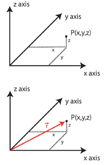
The Cartesian coordinate system applies to three dimensions (as seen in the figure below). The convention is simple:
- The zero point, x = y = z = 0 or (0,0,0), is arbitrary.
- x increases to the east; x decreases to the west.
- y increases to the north; y decreases to the south.
- z increases going up; z decreases going down.
- A distance vector extending from the origin to (x,y,z) as L = i x + j y + k z.
Unit vectors (length 1 along standard coordinates) are i (east); j (north); k (up).
Often we will consider motion in two dimensions as being separate from motions in the vertical. We usually denote the horizontal with a subscript H; for example, LH = i x + j y, where LH is a horizontal distance vector.
We like this coordinate system because it works well over relatively small scales on Earth, perhaps the size of an individual state, where Earth's curvature is not important. However, it does not work so well for large-scale motion on Earth, which is spherical.


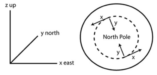
When we place the Cartesian coordinate system on a sphere, note that x always points toward the east, y always points toward the North Pole, and z always points up along the direction of Earth’s radius (as seen in the figure above).
Spherical Coordinate System
Life would be much easier if the Earth were flat. We could then use the Cartesian coordinate system with no worries. But the Earth is a sphere, which implies that to accurately describe motion, we must take the Earth’s spherical shape into account.

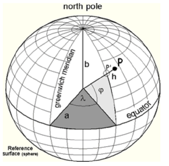
We use the following terms:
- r = distance from the center of the Earth
- \(\Phi=\) latitude \(\left(-90^{\circ} \text { to }+90^{\circ}, \text { or }-\pi / 2 \mathrm{to}+\pi / 2\right)\)
- \(\lambda=\) longitude \(\left(-180^{\circ} \text { to } 180^{\circ}, \text { or }-\pi \text { to }+\pi\right)\)
- State College \(\mathrm{PA}\) is at \(\Phi=40.8^{\circ}\) and \(\lambda=-77.9^{\circ}\)
Note that 1o of latitude is always 111 km or 60 nautical miles, but 1o of longitude is 111 km only at the equator. It is smaller in general and equal to 111 km x cos(Φ). Note that 1 nm = 1.15 miles.
To find the horizontal distance between any two points on Earth's surface, we first need to find the angle of the arc between them and then we can multiply this angle by Earth's radius to get the distance. To find the angle of the arc, \(\Delta \sigma\) , we can use the Spherical Law of Cosines:
\(\Delta \sigma=\arccos \left(\sin \phi_{1} \cdot \sin \phi_{2}+\cos \phi_{1} \cdot \cos \phi_{2} \cdot \cos \Delta \lambda\right)\)
where the latitude and longitude of the two points are \(\Phi_{1}, \lambda_{1}\) and \(\Phi_{2}, \lambda_{2}\) respectively and \(\Delta \lambda=\left|\lambda_{1}-\lambda_{2}\right|\) is the absolute difference between the longitudes of the two points. Note that the angle of the arc must be in radians, where 2\(\pi\) radians \(=360^{\circ} .\) To find the distance, simply multiply this arc angle by the radius of the Earth, 6371 km.
Exercise
Show that 1o of latitude = 111 km distance.
- Click for answer
-
Distance = 6371 km * (1/360)*2π = 111.2 km
In summary, we will use a Cartesian coordinate system when our scales of interest are not too large (synoptic scale or smaller), but will need to use spherical coordinates when the scale of interest is larger than synoptic scale.
For another explanation of these two systems, visit this Coordinate Systems website.
Vertical Coordinates
Three different vertical coordinates are used in meteorology and atmospheric science: height, pressure, and potential temperature.
We have already introduced the vertical coordinate z, which is a height, usually in m or km, above the Earth's surface in the Cartesian coordinate system; z is related to r in spherical coordinates through r = a + z, where a is the Earth's radius. The vertical coordinate z is the most commonly used in meteorology and in any process that involves getting off the ground, such as flight. Often pilots talk about flight levels, which are measured in hundreds of feet. So, flight level 330 is about 10 km altitude.
Another useful vertical coordinate is pressure, which decreases with height. Pressure is often a useful vertical coordinate for calculating dynamics. To a good approximation, pressure falls off exponentially with height,
\[p = p_o\exp(-z/H)\]
so that ln(p) is fairly linear with height. We’ll get into this in greater detail later. For now, consider the following table of typically used pressure heights:
| altitude (km) | altitude (kft) | pressure level (hPa or mb) |
|---|---|---|
| 0 | 0 | 1000 |
| 1.5 | 4.4 | 850 |
| 3.0 | 9.9 | 700 |
| 5.5 | 18.3 | 500 |
A third important vertical coordinate is potential temperature, θ (Equation 2.58). This quantity is the temperature that an air parcel would have if it were brought to a pressure of 1000 hPa without any exchange of heat with its surroundings. This vertical coordinate has a nice property: air parcels tend to move on surfaces of constant potential temperature because moving on such a surface requires no energy. This coordinate is particularly useful in the stratosphere, where the rapid increase with altitude tends to keep air motion stratified.


