2.5: Adiabatic Processes - The Path of Least Resistance
- Page ID
- 3359
\( \newcommand{\vecs}[1]{\overset { \scriptstyle \rightharpoonup} {\mathbf{#1}} } \)
\( \newcommand{\vecd}[1]{\overset{-\!-\!\rightharpoonup}{\vphantom{a}\smash {#1}}} \)
\( \newcommand{\dsum}{\displaystyle\sum\limits} \)
\( \newcommand{\dint}{\displaystyle\int\limits} \)
\( \newcommand{\dlim}{\displaystyle\lim\limits} \)
\( \newcommand{\id}{\mathrm{id}}\) \( \newcommand{\Span}{\mathrm{span}}\)
( \newcommand{\kernel}{\mathrm{null}\,}\) \( \newcommand{\range}{\mathrm{range}\,}\)
\( \newcommand{\RealPart}{\mathrm{Re}}\) \( \newcommand{\ImaginaryPart}{\mathrm{Im}}\)
\( \newcommand{\Argument}{\mathrm{Arg}}\) \( \newcommand{\norm}[1]{\| #1 \|}\)
\( \newcommand{\inner}[2]{\langle #1, #2 \rangle}\)
\( \newcommand{\Span}{\mathrm{span}}\)
\( \newcommand{\id}{\mathrm{id}}\)
\( \newcommand{\Span}{\mathrm{span}}\)
\( \newcommand{\kernel}{\mathrm{null}\,}\)
\( \newcommand{\range}{\mathrm{range}\,}\)
\( \newcommand{\RealPart}{\mathrm{Re}}\)
\( \newcommand{\ImaginaryPart}{\mathrm{Im}}\)
\( \newcommand{\Argument}{\mathrm{Arg}}\)
\( \newcommand{\norm}[1]{\| #1 \|}\)
\( \newcommand{\inner}[2]{\langle #1, #2 \rangle}\)
\( \newcommand{\Span}{\mathrm{span}}\) \( \newcommand{\AA}{\unicode[.8,0]{x212B}}\)
\( \newcommand{\vectorA}[1]{\vec{#1}} % arrow\)
\( \newcommand{\vectorAt}[1]{\vec{\text{#1}}} % arrow\)
\( \newcommand{\vectorB}[1]{\overset { \scriptstyle \rightharpoonup} {\mathbf{#1}} } \)
\( \newcommand{\vectorC}[1]{\textbf{#1}} \)
\( \newcommand{\vectorD}[1]{\overrightarrow{#1}} \)
\( \newcommand{\vectorDt}[1]{\overrightarrow{\text{#1}}} \)
\( \newcommand{\vectE}[1]{\overset{-\!-\!\rightharpoonup}{\vphantom{a}\smash{\mathbf {#1}}}} \)
\( \newcommand{\vecs}[1]{\overset { \scriptstyle \rightharpoonup} {\mathbf{#1}} } \)
\(\newcommand{\longvect}{\overrightarrow}\)
\( \newcommand{\vecd}[1]{\overset{-\!-\!\rightharpoonup}{\vphantom{a}\smash {#1}}} \)
\(\newcommand{\avec}{\mathbf a}\) \(\newcommand{\bvec}{\mathbf b}\) \(\newcommand{\cvec}{\mathbf c}\) \(\newcommand{\dvec}{\mathbf d}\) \(\newcommand{\dtil}{\widetilde{\mathbf d}}\) \(\newcommand{\evec}{\mathbf e}\) \(\newcommand{\fvec}{\mathbf f}\) \(\newcommand{\nvec}{\mathbf n}\) \(\newcommand{\pvec}{\mathbf p}\) \(\newcommand{\qvec}{\mathbf q}\) \(\newcommand{\svec}{\mathbf s}\) \(\newcommand{\tvec}{\mathbf t}\) \(\newcommand{\uvec}{\mathbf u}\) \(\newcommand{\vvec}{\mathbf v}\) \(\newcommand{\wvec}{\mathbf w}\) \(\newcommand{\xvec}{\mathbf x}\) \(\newcommand{\yvec}{\mathbf y}\) \(\newcommand{\zvec}{\mathbf z}\) \(\newcommand{\rvec}{\mathbf r}\) \(\newcommand{\mvec}{\mathbf m}\) \(\newcommand{\zerovec}{\mathbf 0}\) \(\newcommand{\onevec}{\mathbf 1}\) \(\newcommand{\real}{\mathbb R}\) \(\newcommand{\twovec}[2]{\left[\begin{array}{r}#1 \\ #2 \end{array}\right]}\) \(\newcommand{\ctwovec}[2]{\left[\begin{array}{c}#1 \\ #2 \end{array}\right]}\) \(\newcommand{\threevec}[3]{\left[\begin{array}{r}#1 \\ #2 \\ #3 \end{array}\right]}\) \(\newcommand{\cthreevec}[3]{\left[\begin{array}{c}#1 \\ #2 \\ #3 \end{array}\right]}\) \(\newcommand{\fourvec}[4]{\left[\begin{array}{r}#1 \\ #2 \\ #3 \\ #4 \end{array}\right]}\) \(\newcommand{\cfourvec}[4]{\left[\begin{array}{c}#1 \\ #2 \\ #3 \\ #4 \end{array}\right]}\) \(\newcommand{\fivevec}[5]{\left[\begin{array}{r}#1 \\ #2 \\ #3 \\ #4 \\ #5 \\ \end{array}\right]}\) \(\newcommand{\cfivevec}[5]{\left[\begin{array}{c}#1 \\ #2 \\ #3 \\ #4 \\ #5 \\ \end{array}\right]}\) \(\newcommand{\mattwo}[4]{\left[\begin{array}{rr}#1 \amp #2 \\ #3 \amp #4 \\ \end{array}\right]}\) \(\newcommand{\laspan}[1]{\text{Span}\{#1\}}\) \(\newcommand{\bcal}{\cal B}\) \(\newcommand{\ccal}{\cal C}\) \(\newcommand{\scal}{\cal S}\) \(\newcommand{\wcal}{\cal W}\) \(\newcommand{\ecal}{\cal E}\) \(\newcommand{\coords}[2]{\left\{#1\right\}_{#2}}\) \(\newcommand{\gray}[1]{\color{gray}{#1}}\) \(\newcommand{\lgray}[1]{\color{lightgray}{#1}}\) \(\newcommand{\rank}{\operatorname{rank}}\) \(\newcommand{\row}{\text{Row}}\) \(\newcommand{\col}{\text{Col}}\) \(\renewcommand{\row}{\text{Row}}\) \(\newcommand{\nul}{\text{Nul}}\) \(\newcommand{\var}{\text{Var}}\) \(\newcommand{\corr}{\text{corr}}\) \(\newcommand{\len}[1]{\left|#1\right|}\) \(\newcommand{\bbar}{\overline{\bvec}}\) \(\newcommand{\bhat}{\widehat{\bvec}}\) \(\newcommand{\bperp}{\bvec^\perp}\) \(\newcommand{\xhat}{\widehat{\xvec}}\) \(\newcommand{\vhat}{\widehat{\vvec}}\) \(\newcommand{\uhat}{\widehat{\uvec}}\) \(\newcommand{\what}{\widehat{\wvec}}\) \(\newcommand{\Sighat}{\widehat{\Sigma}}\) \(\newcommand{\lt}{<}\) \(\newcommand{\gt}{>}\) \(\newcommand{\amp}{&}\) \(\definecolor{fillinmathshade}{gray}{0.9}\)Adiabatic Process
So far, we have covered constant volume (isochoric) and constant pressure (isobaric) processes. There is a third process that is very important in the atmosphere—the adiabatic process. Adiabatic means no energy exchange between the air parcel and its environment: Q = 0. Note: adiabatic is not the same as isothermal.
Consider the Ideal Gas Law:
\[
p V=n R^{*} T
\]
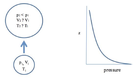
If an air parcel rises, the pressure changes, but how does the temperature change? Note that the volume can change as well as the pressure and temperature, and thus, if we specify a pressure change, we cannot find the temperature change unless we know how the volume changed. Without some other equation, we cannot say how much the temperature will rise for a pressure change.

However, we can use the First Law of Thermodynamics to relate changes in temperature to changes in pressure and volume for adiabatic processes.
Derivation of the Poisson Relations
I do not expect you to be able to do this derivation, but you should go through it to make sure that you understand all the steps as a way to continue to improve your math skills. Start with the following specific form of the 1st Law for dry air:
\[
q=c_{p} \dfrac{d T}{d t}-\alpha \dfrac{d p}{d t}
\]
\[
q=0=c_{p} \dfrac{d T}{d t}-\alpha \dfrac{d p}{d t}
\]
Divide both sides by \(T\) and note that This equation is not rendering properly due to an incompatible browser. See Technical Requirements in the Orientation for a list of compatible browsers. (\(α\) is called the specific volume):
\[
\dfrac{c_{p}}{T} \dfrac{d T}{d t}-\dfrac{R_{d} T}{p T} \dfrac{d p}{d t}=0=\dfrac{c_{p}}{T} \dfrac{d T}{d t}-\dfrac{R_{d}}{p} \dfrac{d p}{d t}=c_{p} \dfrac{d \ln (T)}{d t}-R_{d} \dfrac{d \ln (p)}{d t}
\]
where we figured out the two terms were just derivatives of the natural log of \(T\) and \(p\).
\[
\dfrac{d}{d t}\left(c_{p} \ln (T)-R_{d} \ln (p)\right)=0
\]
But d/dt = 0 just means that the value is constant:
\[
\left(c_{p} \ln (T)-R_{d} \ln (p)\right)=\text { constant }
\]
Divide by cp:
\[
\ln (T)-\dfrac{R_{d}}{c_{p}} \ln (p)=\ln (T)+\ln \left(p^{\left(-R_{d} / c_{p}\right)}\right)=\ln \left(T p^{\left(-R_{d} / c_{p}\right)}\right)=\text {constant }
\]
If the natural log of a variable is constant then the variable itself must be constant:
\[
T p^{\left(-R_{d} / c_{p}\right)}=\text { constant }
\]
We can rewrite Rd/cp as a new term denoted by the Greek letter gamma, \(γ\)
\[
\gamma \equiv \dfrac{c_{p}}{c_{v}}=\dfrac{c_{v}+R_{d}}{c_{v}}=1.4
\]\[
\dfrac{R_{d}}{c_{p}}=\dfrac{\gamma-1}{\gamma}=0.286
\]
We can use the Ideal Gas Law to get relations among p, V, and T, called the Poisson’s Relations:
\[
T p^{\left(-R_{d} / \sigma_{p}\right)}=T p^{((1-n) / r)}=\text { constant }
\]
\[
\alpha^{\gamma} p=\text { constant }
\]
\[
T \alpha^{\gamma-1}=\text {constant }
\]
Potential Temperature
The Poisson Relation that we use the most is the relation of pressure and temperature because these are two variables that we can measure easily without having to define a volume of air:
\[\dfrac{T}{\theta}=\left(\dfrac{p}{p_{o}}\right)^{\left(-R_{d} / c_{p}\right)}\]
or
\[\theta=T\left(\dfrac{p_{o}}{p}\right)^{R_{d} / c_{p}}=T\left(\dfrac{1000}{p}\right)^{0.286}\]
We call θ the potential temperature, which is the temperature that an air parcel would have if the air is brought to a pressure of po = 1000 hPa. Potential temperature is one of the most important thermodynamic quantities in meteorology.
Adiabatic processes are common in the atmosphere, especially the dry atmosphere. Also, adiabatic processes are often the same as isentropic processes (no change in entropy).
Air coming over the Laurel Highlands descends from about 700 m (p ~ 932 hPa) to 300 m (p ~ 977 hPa) at State College. Assume that the temperature in the Laurel Highlands is 20 oC. What is the temperature in State College?
- Click for answer.
-
We can find the temperature in State College due only to adiabatic changes by the following equation:
\(T_{700} p_{700}-0.286=T_{300} p_{300}-0.286\)
\(T_{300=} T_{700}\left(\dfrac{p_{300}}{p_{700}}\right)^{0.286}=(273+20)\left(\dfrac{977}{932}\right)^{0.286}=297 K=24 C\)This temperature change is 4 oC, or 7 oF just from adiabatic compression.
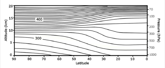
We can plot adiabatic (isentropic) surfaces in the atmosphere. An air parcel needs no energy to move along an adiabatic surface. Also, it takes energy for an air parcel to move from potential surface to another potential energy surface.

Suppose an air parcel has p = 300 hPa and T = 230 K. How much heating per unit volume of dry air would be needed to increase the potential temperature by 10 K?
- Click for answer.
-
The heating raises the temperature, and the amount of heating required depends on the heat capacity, constant pressure, which depends on the mass of air, or the density times the volume. Let's do the calculation for a volume of air; that way we can use the density.
First we need to find the temperature rise that is the same as a potential temperature rise of 10 K at a pressure of 300 hPa.
\(d \theta=d T\left(\dfrac{1000}{p}\right)^{0.286} \quad d T=10\left(\dfrac{300}{1000}\right)^{0.286}=7.1 K\)
Then we need to find the density so that we can calculate the heat capacity:
\(\rho=\dfrac{p}{R_{d} T}=\dfrac{3 \times 10^{4}}{287 \cdot 230}=0.45 \mathrm{kg} m^{-3}\)
Now we can put it all together:
\(\dfrac{Q \Delta t}{V}=\dfrac{\rho \cdot V \cdot c_{p} \cdot \Delta T}{V} \Rightarrow \dfrac{Q \Delta t}{V}=\rho \cdot c_{p} \cdot \Delta T=0.45 \cdot 1005 \cdot 7.1=3.2 x 10^{3} J m^{-3}\)
Note that we were asked to provide the total heating per unit volume, which is just the heating rate times time divided by the unit volume. So the quantity on the left is what we want. Is this heating large? Yes! So it takes a lot of heating or cooling the raise or lower an air parcel potential temperature just 10 K.
Dry Adiabatic Lapse Rate
The temperature change with change in pressure (and thus change in altitude) is a major reason for weather. For dry air, the main effect is buoyancy. So because the pressure change generally follows the hydrostatic equation, the change in height translates into a change in pressure which translates into a change in temperature due to adiabatic expansion. Note that as the air parcel rises, its pressure quickly adjusts to the pressure of the surrounding air. Thus we can determine the dry adiabatic lapse rate by starting with the Poisson relation between pressure and temperature:
\[T p^{\left(^{-R_{d}} / c_{p}\right)}= constant\]
Take the derivative w.r.t. z:
\[\dfrac{d T}{d z} p^{\left(-R_{d} / c_{p}\right)}+T\left(-R_{d} / c_{p}\right) p^{\left(-R_{d} / c_{p}\right)-1} \dfrac{d p}{d z}=\dfrac{d T}{d z}+T\left(-R_{d} / c_{p}\right) p^{-1} \dfrac{d p}{d z}=0\]
But we also know from the hydrostatic equation that:
\[\dfrac{d p}{d z}=-\rho g\]
Substituting –ρg for dp/dz into the equation and rearranging the terms:
\[\dfrac{d T}{d z}=T\left(^{-R_{d}} / c_{p}\right) p^{-1} \rho g=-T\left(R_{d} / c_{p}\right) p^{-1} g\left(\dfrac{p}{R_{d} T}\right)\]
\[-\dfrac{d T}{d z} \equiv \Gamma_{d}=\dfrac{g}{c_{p}}=\dfrac{9.8 \dfrac{m}{s}}{1005 J k g^{-1} K^{-1}}=9.8 K k m^{-1}\]
\(Γ_d\) is called the dry adiabatic lapse rate. Note that the temperature decreases with height, but the dry adiabatic lapse rate is defined as being positive.
Air coming over the Laurel Highlands descends from about 700 m to 300 m at State College. Assume that the temperature in the Laurel Highlands is 20 oC. What is the temperature in State College?
- Click for answer.
-
We can find the temperature in State College due only to adiabatic changes by using the dry adiabatic lapse rate multiplied by the height change:
\(d T=-\Gamma_{d}(300-700)=9.8 K k m^{-1} \cdot 0.4=4^{\circ} C\)
This temperature change is 4.0 oC, or 7 oF just from adiabatic compression. This answer is very similar to the answer we obtained using the change in potential temperature.


