17.11: Canopy Flows

17.11.1. Forests and Crops

The leaf or needle layer of a crop or forest is called a canopy. Individual plants or trees in these crops or forests each cause drag on the wind. The average winds in the air space between these plant-canopy or forest-canopy obstacles is the canopy flow.

Figure 17.40 Canopy flows for (a) crops or urban canopies, and (b) forest canopies having a relatively open trunk space. Left: sketch of the canopy objects. Right: wind profile (solid line). The dashed green line shows a logarithmic profile extrapolated to zero wind speed M. Average top of the canopy is at height h_c.

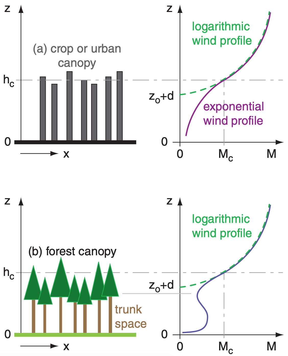
Just above the top of the canopy, the flow is approximately logarithmic with height (Fig. 17.40a). For statically neutral conditions in the surface layer:

\(\ \begin{align}
&M=\frac{u_{*}}{k} \ln \left(\frac{z-d}{z_{o}-d}\right)
&\text { for } z \geq h_{c}
\tag{17.53}\end{align}\)

where M is wind speed, z is height above ground, u* is the friction velocity (a measure of the drag force per unit surface area of the ground), k ≈ 0.4 is the von Kármán constant, d is the displacement distance (0 ≤ d ≤ h_c), and z_o is the roughness length, for an average canopy-top height of h_c.

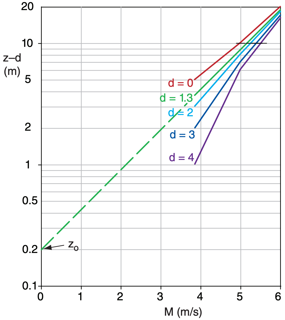
If you can measure the actual wind speed M at 3 or more heights z within 20 m above the top of the canopy, then you can use the following procedure to find d, z_o, and u*: (1) use a spreadsheet to plot your M values on a linear horizontal axis vs. their [z–d] values on a logarithmic vertical axis; (2) experiment with different values of d until you find the one that aligns your wind points into a straight line; (3) extrapolate that straight line to M = 0, and note the resulting intercept on the vertical axis, which gives the roughness length z_o. Finally, (4)pick any point exactly on the plotted line, and then plug in its M and z values, along with the d and z_o values just found, to calculate u* using eq. (17.53).

If you do not have measurements of wind speed above the canopy top, you can use the following crude approximations to estimate the needed parameters: d ≈ 0.65·h_c and z_o ≈ 0.1·h_c. Methods to estimate u* are given in the Boundary-Layer chapter.

The average wind speed at the average canopy-top height is M_c. For the crude approximations above, we find that M_c ≈ 3.13 u*.

Within the top 3/4 of canopy, an exponential formula describes the average wind-speed M profile:

\(\ \begin{align} M=M_{c} \cdot \exp \left[a \cdot\left(\frac{z}{h_{c}}-1\right)\right] \quad \text { for } 0.5 h_{c} \leq z \leq h_{c}\tag{17.54}\end{align}\)

where a is an attenuation coefficient that increases with increasing leaf area and decreases as the mean distance between individual plants increases. Typical values are: a ≈ 2.5 - 2.8 for oats and wheat; 2.0 - 2.7 for mature corn; 1.3 for sunflowers; 1.0 - 1.1 for larch and small evergreen trees; and 0.4 for a citrus orchard. The exponential and log-wind speeds match at the average canopy top h_c.

For a forest with relatively open trunk space (i.e., only the tree trunks without many leaves, branches, or smaller underbrush), the previous equation fails. Instead, a weak relative maximum wind speed can occur (Fig. 17.40b). In such forests, if the canopy is very dense, then the sub-canopy (trunk space) flow can be relatively disconnected from the flow above the tree tops. Weak katabatic flows can exist in the trunk space day and night.

Sample Application (§)

Given these wind measurements over a 2 m high corn crop: [z (m), M (m s^–1)] = [5, 3.87] , [10, 5.0] , [20, 6.01]. Find the displacement distance, roughness length, and friction velocity. If the attenuation coefficient is 2.5, plot wind speed M vs. height over 0.5 m ≤ z ≤ 5 m.

Find the Answer

Given: h_c =2m, [z (m), M (m s^–1)] listed above, a = 2.5.

Find: d = ? m, z_o = ? m, u* = ? m s^–1, and plot M vs. z.

Guess d = 0, and plot M vs. log(z–d) on a spreadsheet. This d is too small (see graph below), because the curve is concave up. Guess d = 4, which is too large, because curve is concave down. After other guesses (some not shown), I find that d = 1.3 m gives the straightest line.

Next, extrapolate on the semi-log graph to M = 0, which gives an intercept of z_o = 0.2 m.

Solve eq. (17.53) for u* = k·M/ln[(z–d)/z_o]

u* = 0.4(5m s^–1)/ln[(10–1.3)/0.2] = 0.53 ms^–1

Solve eq. (17.53) for M_c at z = h_c = 2 m:

M_c = [(0.53m s^–1)/0.4] · ln[(2–1.3m)/0.2] = 1.66 m s^–1

Use eq. (17.54) to find M for a range of heights below h_c, and use eq. (17.53) for heights above h_c:

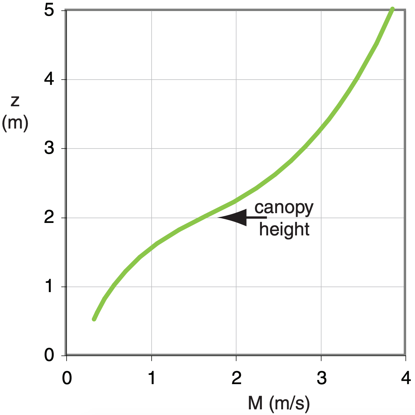
Check: Shape of curve looks reasonable.

Exposition: For this exercise, z_o = 0.1 h_c, and d = 0.65 h_c. Namely, the crude approximations are OK.

17.11.2. Cities

The collection of buildings and trees that make up a city is sometimes called an urban canopy. These obstacles cause an average canopy-flow wind similar to that for forests and crops (Fig. 17.40a).

However, winds at any one location in the city can be quite different. For example, the street corridors between tall buildings can channel flow similar to the flow in narrow valleys. Hence these corridors are sometimes called urban canyons. Also, taller buildings can deflect down to the surface some of the faster winds aloft. This causes much greater wind speeds and gusts near the base of tall buildings than near the base of shorter buildings.

Cities can be 2 - 12°C degrees warmer than the surrounding rural countryside — an effect called the urban heat island (UHI, Fig. 17.41). Reasons include the abundance of concrete, glass and asphalt, which capture and store the solar heat during daytime and reduce the IR cooling at night. Also, vegetated areas are reduced in cities, and rainwater is channeled away through storm drains. Hence, there is less evaporative cooling. Also, fuel and electrical consumption by city residents adds heat via heating, air conditioning, industry, and transportation.

Figure 17.41 An urban heat island at night, where T_o is the rural air temperature. The grid represents city streets.

Figure 17.42 Maximum urban-heat-island temperature difference ∆T_{UHI_ max} increases with average aspect ratio H/W of the urban canyons near the built-up city center. Based on data from North America, Europe, and Australasia. [Adapted from Oke, Mills, Christen, & Voogt, 2016: Urban Climates, submitted to Cambridge Univ. Press. (used with lead author’s permission).]

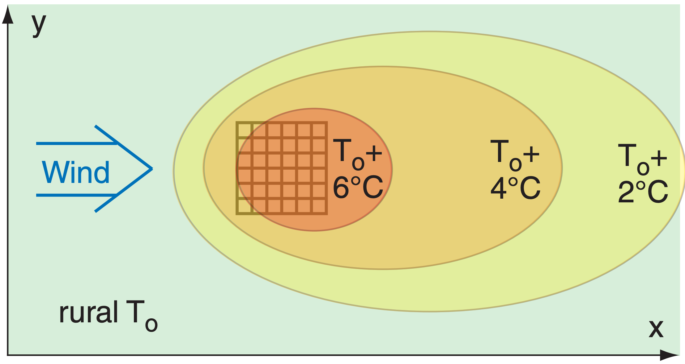
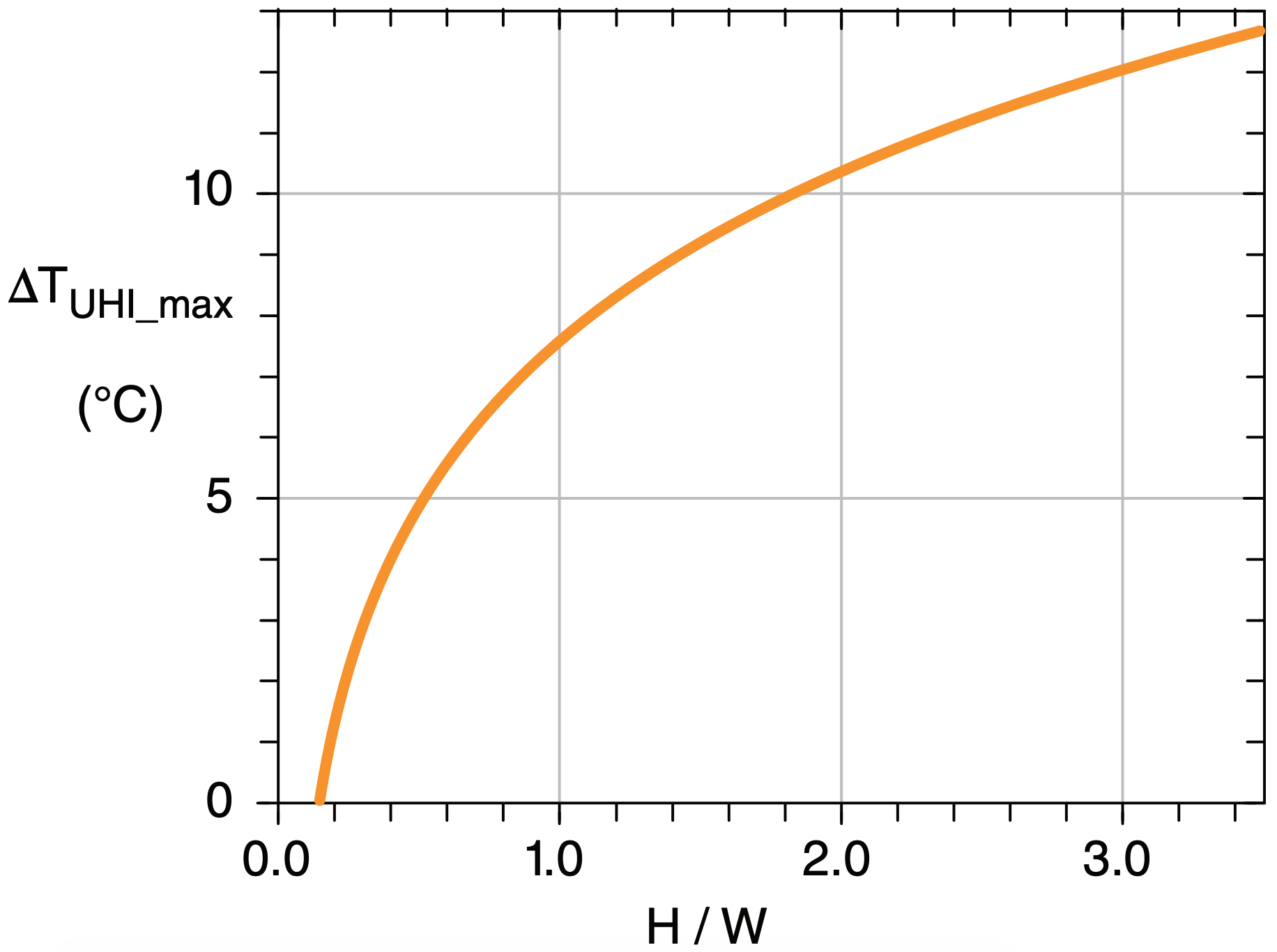
The city–rural temperature difference ∆T_UHI is greatest during clear calm nights, because the city stays warm while rural areas cool considerably due to IR radiation to space. The largest values ∆T_{UHI_ max} occur near the city center (Fig. 17.42), at the location of greatest density of high buildings and narrow streets. For clear, calm nights, this relationship is described by

\(\ \begin{align} \Delta T_{U H I_{-} \max} \approx a+b \cdot \ln (H / W)\tag{17.55}\end{align}\)

where a = 7.54°C and b = 3.97°C. H is the average height (m) of the buildings in the downtown city core, W is the average width (m) of the streets at the same location, and H/W is dimensionless.

Temperature difference is much smaller during daytime. When averaged over a year (including windy and cloudy periods of minimal UHI), the average ∆T_UHI at the city center is only 1 to 2°C.

During periods of fair weather and light synopticscale winds, the warm city can generate circulations similar to sea breezes, with inflow of low-altitude rural air toward the city, and rising air over the hottest parts of town. These circulations can enhance clouds, and trigger or strengthen thunderstorms over and downwind of the city. With light to moderate winds, the UHI area is asymmetric, extending much further from the city in the downwind direction (Fig. 17.41), and the effluent (heat, air pollution, odors) from the city can be observed downwind as an urban plume (Fig. 17.43).