17.2: Wind-Turbine Power Generation

Power is defined as the rate of energy production. Kinetic energy of the wind is proportional to air mass times wind-speed squared. The rate at which this energy is blown through a wind turbine is the wind speed. Thus, the theoretical power available from the wind is proportional to wind speed cubed:

\(\ \begin{align} \text{Power}=(\pi / 2) \cdot p \cdot E \cdot R^{2} \cdot M_{i n}^{3}\tag{17.2}\end{align}\)

where R is the turbine-blade radius, M_in is incoming wind speed, and ρ is air density. Turbine efficiencies are E = 30% to 45%.

Faster winds and larger-radius turbines allow greater power generation. Modern large wind turbines have a hub height (center of the turbine) of 80 m or more, to reach the faster winds higher above the surface. Turbines with radius of 30 m can generate up to 1.5 MW (mega Watts) of electricity, while blades of 40 m radius can generate up to 2.5 MW.

Figure 17.4 Wind turbine for electrical-power generation. Blue region shows the air that enters and leaves the wind turbine.

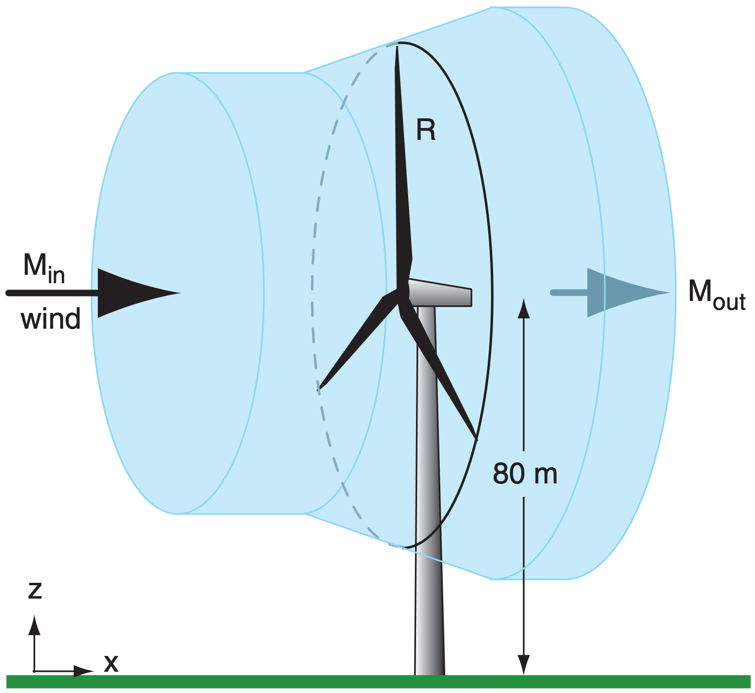
To see how a wind turbine works, consider Fig. 17.4 with an incoming wind speed M_in. Even before the wind reaches the disk swept out by the turbine blades, it feels the increased drag (higher pressure) from the turbine and begins to slow. It slows further while passing through the turbine (because the turbine is extracting energy from the wind), and slows more just behind the turbine due to the suction drag. Because the exit speed M_out is slower than the entrance speed, and because air-volume flow rate (= M · cross-section area) is conserved, the diameter of the air that feels the influence of the turbine must increase as wind speed decreases.

Zero exit speed is impossible, because the exited air would block subsequent in-flow, preventing power production. Also, if the exit speed equals the entrance speed, then power production is zero because no energy is extracted from the wind. Thus, wind turbines are designed to have an optimum wind-speed decrease of M_out/M_in = 1/3 (see HIGH ER MATH box on Betz’ Law). Albert Betz showed that the theoretical maximum turbine efficiency at this optimum speed is E_max = 16/27 = 59.3%, which is known as Betz’ Limit.

Figure 17.5 Typical power-output curve for a 1 MW wind turbine as a function of wind speed M.

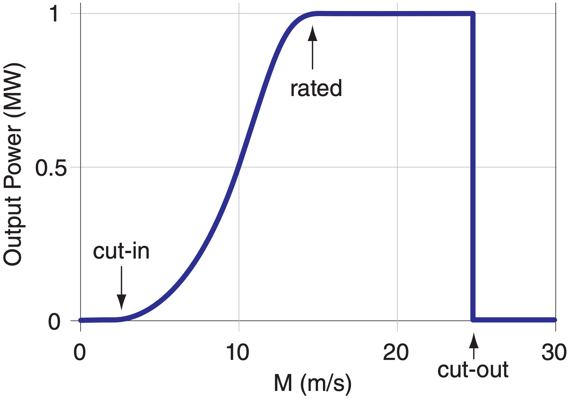
Wind turbines need a wind speed of at least 3 to 5 m s^–1 to start turning. This is called the cutin speed. As wind speed increases, so increases the amount of power generated. At its rated wind speed (8 to 15 m s^–1), the turbine is producing the maximum amount of electricity that the generators can handle. As wind speeds increase further, the aerodynamics of the blades are designed to change (via feathering the blades to reduce their pitch, or causing aerodynamic stalling) to keep the shaft rotation rate and electrical power generation nearly constant. Namely, the efficiency is intentionally reduced to protect the equipment. Finally, for wind speeds at or above a cut-out wind speed (25 - 30 m s^–1), turbine rotation is stopped by feathering (changing the angle of attack of) the blades, to prevent damage. Fig. 17.5 shows the resulting idealized power output curve for a wind turbine.

HIGHER MATH • Betz’ Law

In 1919 Albert Betz reasoned that the energy extracted by the turbine is the difference between incoming and outgoing kinetic energies:

\(\ \begin{align} \text{Energy} =0.5 \cdot m \cdot M_{i n}^{2}-0.5 \cdot m \cdot M_{o u t}^{2}\tag{1}\end{align}\)

where m is air mass and M is wind speed. The amount of air mass moving through the disk swept by the turbine during time interval ∆t is the air density ρ times disk area (A = πR²) times average speed:

\(\ \begin{align} m=\rho \cdot A \cdot 0.5\left(M_{i n}+M_{o u t}\right) \cdot \Delta t\tag{2}\end{align}\)

Plug this into the previous eq. and divide by ∆t to get the power that the turbine can produce:

\(\ \begin{align} \text{Power} =0.25 \cdot \rho \cdot A \cdot\left(M_{\text {in }}+M_{\text {out }}\right) \cdot\left(M_{\text {in }}^{2}-M_{\text {out }}^{2}\right)\tag{3}\end{align}\)

Divide this power by the power of the incoming wind 0.5·ρ·A· M_in³ to get a theoretical efficiency E_o:

\(\ \begin{align} E_{o}=(1 / 2) \cdot\left[1-\left(M_{o u t} / M_{i n}\right)^{2}\right] \cdot\left[1+\left(M_{o u t} / M_{i n}\right)\right]\tag{4}\end{align}\)

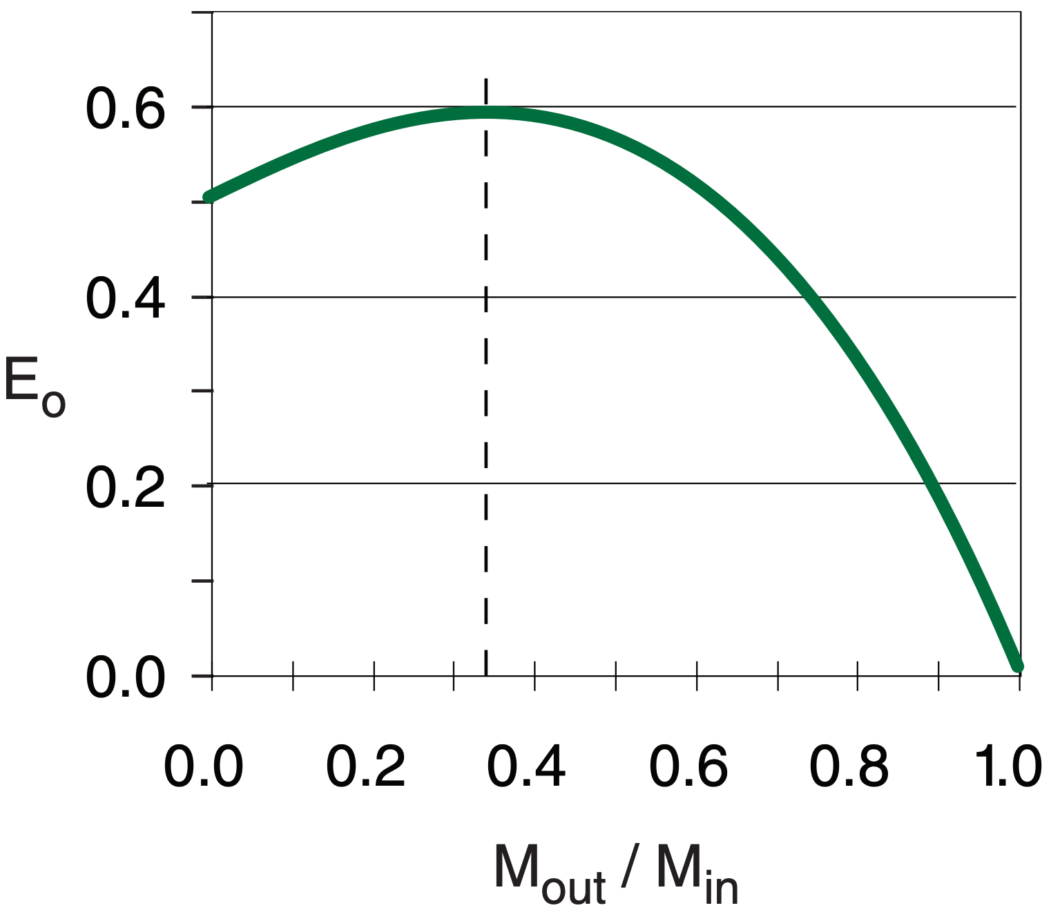
Solve eq. (4) on a spreadsheet and plot E_o vs. M_out/M_in (see Fig. below) The peak in the curve gives

E_max = 0.593 at M_out/M_in = 1/3.

Fig. 17.a Theoretical turbine efficiencies using Betz’ Law.

We can get the precise answer using calculus. Let the ratio of wind speeds be r = M_out/M_in , to simplify the notation. Use r in eq. (4):

\(\ \begin{align} E_{o}=(1 / 2) \cdot\left(1-r^{2}\right) \cdot(1+r)=(1 / 2) \cdot\left[1+r-r^{2}-r^{3}\right]\tag{5}\end{align}\)

Differentiate E_o and set dEo/dr = 0 to find the value of r at max E_o:

\(\ \begin{align} 3 r^{2}+2 r-1=0\tag{6}\end{align}\)

Solving this quadratic eq for r gives r =1/3 and r = –1, for which the only physically reasonable answer is

\(\ r=M_{o u t} / M_{i n}=\underline{\mathbf{1/ 3}}\)

Finally, plug this r into eq. (5) to get the max E_o:

\(\ \begin{align} E_{\max }=(1 / 2) \cdot[1+(1 / 3)-(1 / 9)-(1 / 27)]\tag{7}\end{align}\)

Using a common denominator of 27, we find

\(E_{\max }=(1 / 2) \cdot[32 / 27]=16 / 27=0.593=\underline{\mathbf{5 9.3\%}}\)