
6.7: Fractal Cloud Shapes
- Page ID
- 9934

\( \newcommand{\vecs}[1]{\overset { \scriptstyle \rightharpoonup} {\mathbf{#1}} } \)
\( \newcommand{\vecd}[1]{\overset{-\!-\!\rightharpoonup}{\vphantom{a}\smash {#1}}} \)
\( \newcommand{\dsum}{\displaystyle\sum\limits} \)
\( \newcommand{\dint}{\displaystyle\int\limits} \)
\( \newcommand{\dlim}{\displaystyle\lim\limits} \)
\( \newcommand{\id}{\mathrm{id}}\) \( \newcommand{\Span}{\mathrm{span}}\)
( \newcommand{\kernel}{\mathrm{null}\,}\) \( \newcommand{\range}{\mathrm{range}\,}\)
\( \newcommand{\RealPart}{\mathrm{Re}}\) \( \newcommand{\ImaginaryPart}{\mathrm{Im}}\)
\( \newcommand{\Argument}{\mathrm{Arg}}\) \( \newcommand{\norm}[1]{\| #1 \|}\)
\( \newcommand{\inner}[2]{\langle #1, #2 \rangle}\)
\( \newcommand{\Span}{\mathrm{span}}\)
\( \newcommand{\id}{\mathrm{id}}\)
\( \newcommand{\Span}{\mathrm{span}}\)
\( \newcommand{\kernel}{\mathrm{null}\,}\)
\( \newcommand{\range}{\mathrm{range}\,}\)
\( \newcommand{\RealPart}{\mathrm{Re}}\)
\( \newcommand{\ImaginaryPart}{\mathrm{Im}}\)
\( \newcommand{\Argument}{\mathrm{Arg}}\)
\( \newcommand{\norm}[1]{\| #1 \|}\)
\( \newcommand{\inner}[2]{\langle #1, #2 \rangle}\)
\( \newcommand{\Span}{\mathrm{span}}\) \( \newcommand{\AA}{\unicode[.8,0]{x212B}}\)
\( \newcommand{\vectorA}[1]{\vec{#1}} % arrow\)
\( \newcommand{\vectorAt}[1]{\vec{\text{#1}}} % arrow\)
\( \newcommand{\vectorB}[1]{\overset { \scriptstyle \rightharpoonup} {\mathbf{#1}} } \)
\( \newcommand{\vectorC}[1]{\textbf{#1}} \)
\( \newcommand{\vectorD}[1]{\overrightarrow{#1}} \)
\( \newcommand{\vectorDt}[1]{\overrightarrow{\text{#1}}} \)
\( \newcommand{\vectE}[1]{\overset{-\!-\!\rightharpoonup}{\vphantom{a}\smash{\mathbf {#1}}}} \)
\( \newcommand{\vecs}[1]{\overset { \scriptstyle \rightharpoonup} {\mathbf{#1}} } \)
\(\newcommand{\longvect}{\overrightarrow}\)
\( \newcommand{\vecd}[1]{\overset{-\!-\!\rightharpoonup}{\vphantom{a}\smash {#1}}} \)
\(\newcommand{\avec}{\mathbf a}\) \(\newcommand{\bvec}{\mathbf b}\) \(\newcommand{\cvec}{\mathbf c}\) \(\newcommand{\dvec}{\mathbf d}\) \(\newcommand{\dtil}{\widetilde{\mathbf d}}\) \(\newcommand{\evec}{\mathbf e}\) \(\newcommand{\fvec}{\mathbf f}\) \(\newcommand{\nvec}{\mathbf n}\) \(\newcommand{\pvec}{\mathbf p}\) \(\newcommand{\qvec}{\mathbf q}\) \(\newcommand{\svec}{\mathbf s}\) \(\newcommand{\tvec}{\mathbf t}\) \(\newcommand{\uvec}{\mathbf u}\) \(\newcommand{\vvec}{\mathbf v}\) \(\newcommand{\wvec}{\mathbf w}\) \(\newcommand{\xvec}{\mathbf x}\) \(\newcommand{\yvec}{\mathbf y}\) \(\newcommand{\zvec}{\mathbf z}\) \(\newcommand{\rvec}{\mathbf r}\) \(\newcommand{\mvec}{\mathbf m}\) \(\newcommand{\zerovec}{\mathbf 0}\) \(\newcommand{\onevec}{\mathbf 1}\) \(\newcommand{\real}{\mathbb R}\) \(\newcommand{\twovec}[2]{\left[\begin{array}{r}#1 \\ #2 \end{array}\right]}\) \(\newcommand{\ctwovec}[2]{\left[\begin{array}{c}#1 \\ #2 \end{array}\right]}\) \(\newcommand{\threevec}[3]{\left[\begin{array}{r}#1 \\ #2 \\ #3 \end{array}\right]}\) \(\newcommand{\cthreevec}[3]{\left[\begin{array}{c}#1 \\ #2 \\ #3 \end{array}\right]}\) \(\newcommand{\fourvec}[4]{\left[\begin{array}{r}#1 \\ #2 \\ #3 \\ #4 \end{array}\right]}\) \(\newcommand{\cfourvec}[4]{\left[\begin{array}{c}#1 \\ #2 \\ #3 \\ #4 \end{array}\right]}\) \(\newcommand{\fivevec}[5]{\left[\begin{array}{r}#1 \\ #2 \\ #3 \\ #4 \\ #5 \\ \end{array}\right]}\) \(\newcommand{\cfivevec}[5]{\left[\begin{array}{c}#1 \\ #2 \\ #3 \\ #4 \\ #5 \\ \end{array}\right]}\) \(\newcommand{\mattwo}[4]{\left[\begin{array}{rr}#1 \amp #2 \\ #3 \amp #4 \\ \end{array}\right]}\) \(\newcommand{\laspan}[1]{\text{Span}\{#1\}}\) \(\newcommand{\bcal}{\cal B}\) \(\newcommand{\ccal}{\cal C}\) \(\newcommand{\scal}{\cal S}\) \(\newcommand{\wcal}{\cal W}\) \(\newcommand{\ecal}{\cal E}\) \(\newcommand{\coords}[2]{\left\{#1\right\}_{#2}}\) \(\newcommand{\gray}[1]{\color{gray}{#1}}\) \(\newcommand{\lgray}[1]{\color{lightgray}{#1}}\) \(\newcommand{\rank}{\operatorname{rank}}\) \(\newcommand{\row}{\text{Row}}\) \(\newcommand{\col}{\text{Col}}\) \(\renewcommand{\row}{\text{Row}}\) \(\newcommand{\nul}{\text{Nul}}\) \(\newcommand{\var}{\text{Var}}\) \(\newcommand{\corr}{\text{corr}}\) \(\newcommand{\len}[1]{\left|#1\right|}\) \(\newcommand{\bbar}{\overline{\bvec}}\) \(\newcommand{\bhat}{\widehat{\bvec}}\) \(\newcommand{\bperp}{\bvec^\perp}\) \(\newcommand{\xhat}{\widehat{\xvec}}\) \(\newcommand{\vhat}{\widehat{\vvec}}\) \(\newcommand{\uhat}{\widehat{\uvec}}\) \(\newcommand{\what}{\widehat{\wvec}}\) \(\newcommand{\Sighat}{\widehat{\Sigma}}\) \(\newcommand{\lt}{<}\) \(\newcommand{\gt}{>}\) \(\newcommand{\amp}{&}\) \(\definecolor{fillinmathshade}{gray}{0.9}\) Fractals are patterns made of the superposition of similar shapes having a range of sizes. An example is a dendrite snow flake. It has arms protruding from the center. Each of those arms has smaller arms attached, and each of those has even smaller arms. Other aspects of meteorology exhibit fractal geometry, including lightning, turbulence, and clouds. Fractals are defined next, and then are applied to cloud shadows.
6.7.1. Fractal Dimension
Euclidean geometry includes only integer dimensions; for example 1-D, 2-D or 3-D. Fractal geometry allows a continuum of dimensions; for example D = 1.35 .
Fractal dimension is a measure of space-filling ability. Common examples are drawings made by children, and newspaper used for packing cardboard boxes.
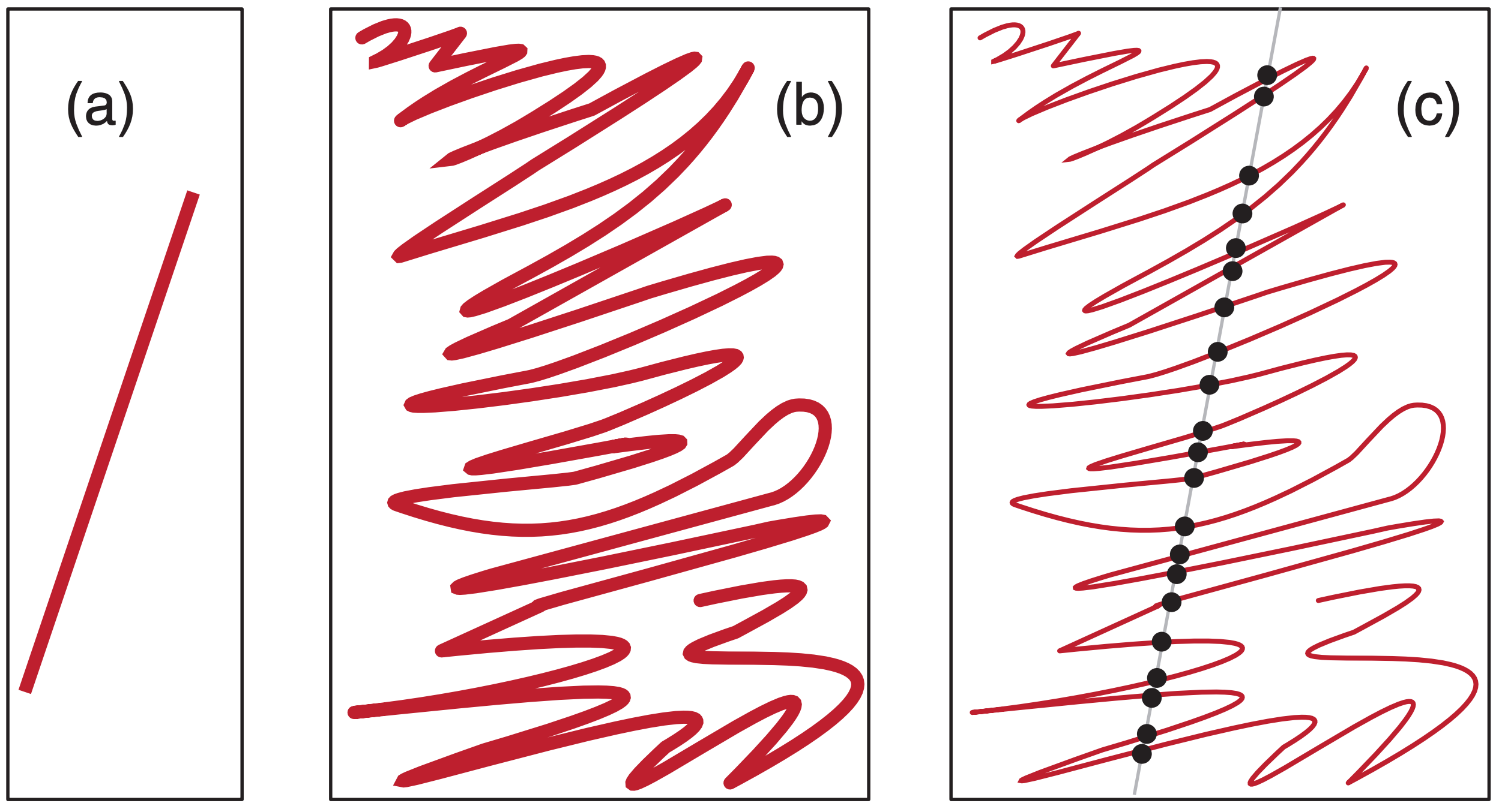
A straight line (Figure 6.11a) has fractal dimension D = 1; namely, it is one-dimensional both in the Euclidean and fractal geometry. When toddlers draw with crayons, they fill areas by drawing tremendously wiggly lines (Figure 6.11b). Such a line might have fractal dimension D ≈ 1.7, and gives the impression of almost filling an area. Older children succeed in filling the area, resulting in fractal dimension D = 2.
A different example is a sheet of newspaper. While it is flat and smooth, it fills only two-dimensional area (neglecting its thickness), hence D = 2. However, it takes up more space if you crinkle it, resulting in a fractal dimension of D ≈ 2.2. By fully wadding it into a tight ball of D ≈ 2.7, it begins to behave more like a three-dimensional object, which is handy for filling empty space in cardboard boxes.
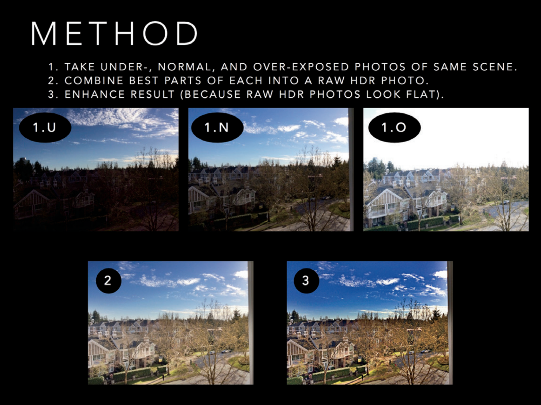 Most people take photos with their cell phone or tablet. You cannot easily add special lenses and filters to these devices. Instead, to take better cloud photos, use special software on your device to capture high dynamic range (HDR) images.
When you take an HDR photo, your camera takes three photos in rapid succession of the same scene. One photo uses a good average exposure for the whole scene (1.N). Another is underexposed (1.U), but captures the sky and clouds better. The third is overexposed (1.O), to capture darker ground and shadows. The software automatically combines the best parts of the three photos into one photo (2). Finally, after you enhance the saturation, contrast, and sharpness, the image (3) is much better than the normal photo (1.N).
A zero set is a lower-dimensional slice through a higher-dimensional shape. Zero sets have fractal dimension one less than that of the original shape (i.e., Dzero set = D – 1). Sometimes it is easier to measure the fractal dimension of a zero set, from which we can calculate the dimension of the original.
For example, start with the wad of paper having fractal dimension D = 2.7. It would be difficult to measure the dimension for this wad of paper. Instead, carefully slice that wad into two halves, dip the sliced edge into ink, and create a print of that inked edge on a flat piece of paper. The wiggly line that was printed (Figure 6.11b) has fractal dimension of D = 2.7 – 1 = 1.7, and is a zero set of the original shape. It is easier to measure.
To continue the process, slice through the middle of the print (shown as the grey line in Figure 6.11c). The wiggly printed line crosses the straight slice at a number of points (Figure 6.11c); those points have a fractal dimension of D = 1.7 – 1 = 0.7, and represent the zero set of the print. Thus, while any one point has a Euclidean dimension of zero, the set of points appears to partially fill a 1-D line.
6.7.2. Measuring Fractal Dimension
Consider an irregular-shaped area, such as the shadow of a cloud. The perimeter of the shadow is a wiggly line, so we should be able to measure its fractal dimension. Based on observations of the perimeter of real-cloud shadows, D = 1.35 . If we assume that this cloud shadow is a zero set of the surface of the cloud, then the cloud surface dimension is D = Dzero set + 1 = 2.35. The fractal nature of clouds suggests that some turbulent or chaotic dynamics might need to be considered when modeling clouds.
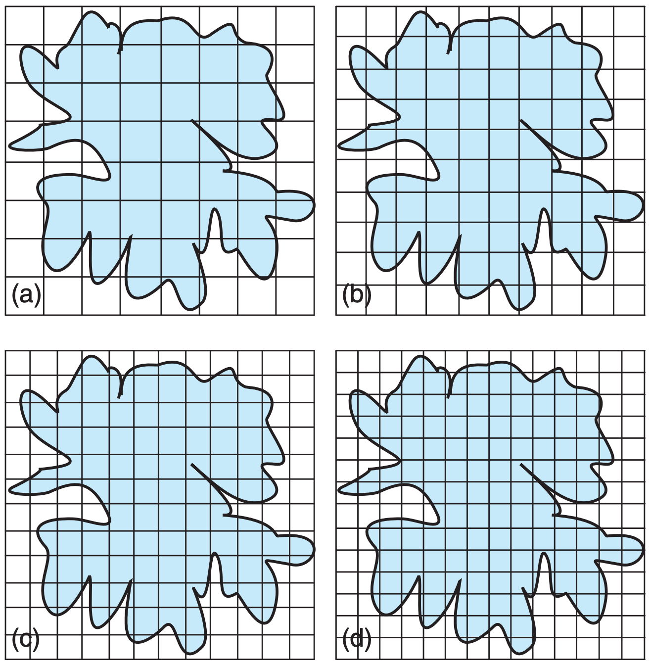
A box-counting method can be used to measure fractal dimension. Put the cloud-shadow picture within a square domain. Then tile the domain with smaller square boxes, with M tiles per side of domain (Figure 6.12). Count the number N of tiles through which the perimeter passes. Repeat the process with smaller tiles.
Get many samples of N vs. M, and plot these as points on a log-log graph. The fractal dimension D is the slope of the best fit straight line through the points. Define subscripts 1 and 2 as the two end points of the best fit line. Thus:
\(\ \begin{align} D=\dfrac{\log \left(N_{1} / N_{2}\right)}{\log \left(M_{1} / M_{2}\right)}\tag{6.7}\end{align}\)
This technique works best when the tiles are small. If the plotted line is not straight but curves on the log-log graph, try to find the slope of the portion of the line near large M.
Sample Application
Use Fig. 6.12 to measure the fractal dimension of the cloud shadow.
Find the Answer
For each figure, the number of boxes is:
| M | N | |
| (a) | 8 | 44 |
| (b) | 10 | 53 |
| (c) | 12 | 75 |
| (d) | 14 | 88 |
(You might get a slightly different count.)
Plot the result on a log-log graph, & fit a straight line.
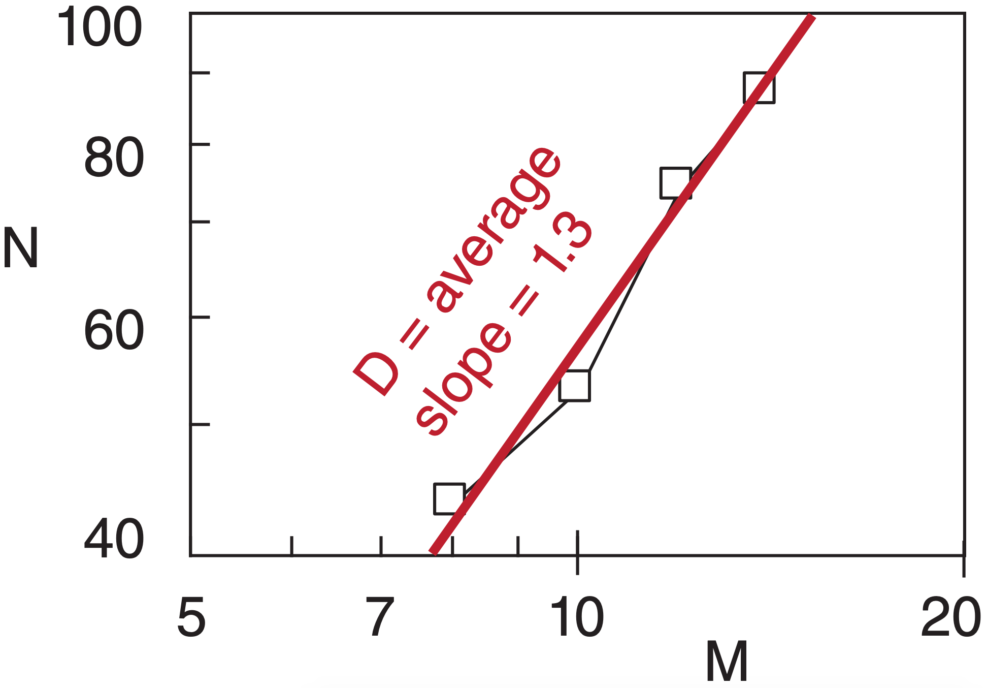
Use the end points of the best-fit line in eq. (6.7):
\(D=\dfrac{\log (100 / 40)}{\log (15 / 7.5)}=1.32\)
Check: Units OK. Physics OK.
Exposition: About right for a cloud. The original domain size relative to cloud size makes no difference. Although you will get different M and N values, the slope D will be almost the same.