8.2: Weather Radars

8.3.1. Fundamentals

Weather radars are active sensors that emit pulses of very intense (250 - 1000 kW) microwaves generated by magnetron or klystron vacuum tubes. These transmitted pulses, each of ∆t = 0.5 to 10 µs duration, are reflected off a parabolic antenna dish. The dish can rotate and tilt to point the train of pulses toward any azimuth and elevation angle in the atmosphere. Pulse repetition frequencies (PRF) are on the order of 50 to 2000 pulses per second.

Figure 8.22: Radar beam. MUR is maximum unambiguous range.

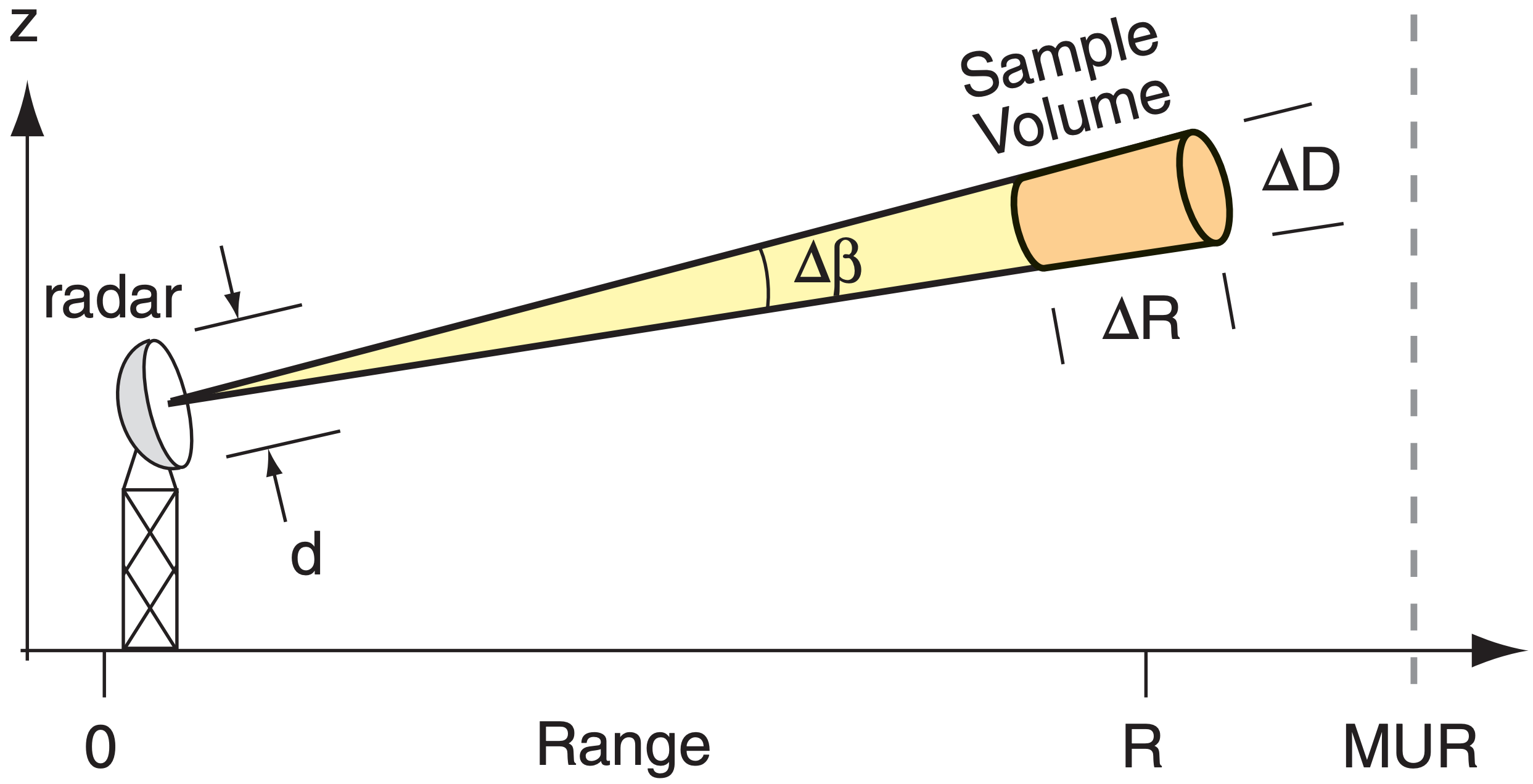
The microwaves travel away from the radar at the speed of light through the air (c ≈ 3x10⁸ m s^–1), focused by the antenna dish along a narrow beam (Fig. 8.22). The angular thickness of this beam, called the beamwidth \(Δβ\), depends on the wavelength λ of the microwaves and the diameter (\(d\)) of the parabolic antenna:

\(\ \begin{align} \Delta \beta=a \cdot \lambda / d\tag{8.13}\end{align}\)

where a = 71.6°. Larger-diameter antennae can focus the beam into narrower beamwidths. For many weather radars, Δβ < 1°.

Sample Application

Given a 10 cm wavelength radar with a 9 m diameter antenna dish, find the beamwidth.

Find the Answer

Given: λ = 10 cm = 0.1 m , d = 9 m.

Find: Δβ = ?°

Use eq. (8.13): Δβ = (71.6°)·(0.1m)/(9m) = 0.8°

Check: Units OK. Physics OK. Reasonable value.

Exposition: This large dish and wavelength are used for the USA WSR-88D operational weather radars.

The volume sampled by any one pulse is shaped like a slightly tapered cylinder (i.e., the frustum of a cone; shaded in Fig. 8.22). Typical pulse lengths (c·∆t) are 300 to 500 m. However, the sampled length ∆R is half the pulse length, because of the round trip the energy must travel in and out of the sample volume.

\(\ \begin{align} \Delta R=c \cdot \Delta t / 2\tag{8.14}\end{align}\)

The diameter (∆D) is:

\(\ \begin{align} \Delta D=R \cdot \Delta \beta\tag{8.15}\end{align}\)

for beamwidth ∆β in radians (= degrees · π/180°). ∆D ≈ 0.1 km at close range (R), and increases to 10 km at far range. Thus, the resolution of the radar decreases as range increases.

A very small amount (10^–5 to 10^–15 W) of the transmitted energy is scattered back towards the radar when the microwave pulses hit objects such as hydrometeors (rain, snow, hail), insects, birds, aircraft, buildings, mountains, and trees. The radar dish collects these weak returns (echoes) and focuses them onto a detector. The resulting signal is amplified and digitally processed, recorded, and displayed graphically.

The range (radial distance) R from the radar to any target is easily calculated by measuring the round-trip time t between transmission of the pulse and reception of the scattered signal:

\(\ \begin{align} R=c \cdot t / 2\tag{8.16}\end{align}\)

Also, the azimuth and elevation angles to the target are known from the direction the radar dish was pointing when it sent and received the signals. Thus, there is sufficient information to position each target in 3-D space within the volume scanned.

Weather radar cannot “see” each individual rain or cloud drop or ice crystal. Instead, it sees the average energy returned from all the hydrometeors within a finite-sized pulse subvolume. This is analogous to how your eyes see a cloud; namely, you can see a white cloud even though you cannot see each individual cloud droplet.

Weather radars look at three characteristics of the returned signal to help detect storms and other conditions: reflectivity, Doppler shift, and polarization. These will be explained in detail, after first covering a few more radar fundamentals.

Sample Application

Find the round-trip travel time to a target at R=20 km.

Find the Answer

Given: R = 20 km = 2x10⁴ m, c = 3 x 10⁸ m s^–1.

Find: t = ? µs

Rearrange eq. (8.16): t = 2 R / c

t = 2 ·(2x10⁴m) / (3x10⁸m s^–1) = 1.33x10^–4 s = 133 µs

Check: Units OK. Physics OK.

Exposition: The typical duration of an eye blink is 100 to 200 ms. Thus, the radar pulse could make 1000 round trips to 20 km in the blink of an eye.

8.3.1.1. Maximum Range

The maximum range that the radar can “see” is limited by both the attenuation (absorption of the microwave energy by intervening hydrometeors) and pulse-repetition frequency. In heavy rain, so much of the radar energy is absorbed and scattered that little can propagate all the way through (recall Beer’s Law from the Radiation chapter). The resulting radar shadows behind strong targets are “blind spots” that the radar can’t see.

Even with little attenuation, the radar can “listen” for the return echoes from one transmitted pulse only up until the time the next pulse is transmitted. For those radars where the microwaves are generated by klystron tubes (for which every pulse has exactly the same frequency, amplitude, and phase), any echoes received after this time are erroneously assumed to have come from the second pulse. Thus, any target greater than this maximum unambiguous range (MUR, or R_max) would be erroneously displayed a distance R_max closer to the radar than it actually is (Fig. 8.35a). MUR is given by:

\[\ \begin{align} R_{\max }=c /[2 \cdot P R F]\tag{8.17}\end{align}\]

Magnetron tubes produce a more random signal that varies from pulse to pulse, which can be used to discriminate between subsequent pulses and their return signals, thereby avoiding the MUR problem.

Sample Application

A 5 cm wavelength radar with 5 m diameter antenna dish transmits 1000 pulses per second, each pulse lasting 1 µs. (a) What are the sample-volume dimensions for a pulse received 100 µs after transmission? (b) Is the range to this sample volume unambiguous?

Find the Answer

Given: λ = 5 cm, d = 5 m, PRF = 1000 s^–1, ∆t = 1 µs, t = 100 µs.

Find: (a) ∆R = ? m, and ∆D = ? m. (b) R_max = ? km.

(a) Use eq. (8.14): ∆R = (3x10⁸m/s)·(10^–6s)/2 = 150 m.

To use eq. (8.15) for ∆D, we first need R and Δβ .

From eq. (8.13): Δβ = (71.6°)·(0.05m)/(5m) = 0.72°

From eq. (8.16): R = (3x10⁸m/s)·(10^–4s)/2 = 15 km.

Use eq. (8.15): ∆D = (15000m)·(0.72°)·π/(180°)= 188 m.

(b) Use eq. (8.17): R_max=(3x10⁸m/s)/[2·1000 s^–1]=150km

But R = 15 km from (a).

Yes, range IS unambiguous because R < Rmax .

Check: Units OK. Physics OK.

Exposition: If the range to the rain shower had been R = 160 km, then the target would have appeared on the radar display at an erroneous range of R – R_max = 160 – 150 km = 10 km from the radar, and would be superimposed on any echoes actually at 10 km range.

8.3.1.2. Scan and Display Strategies

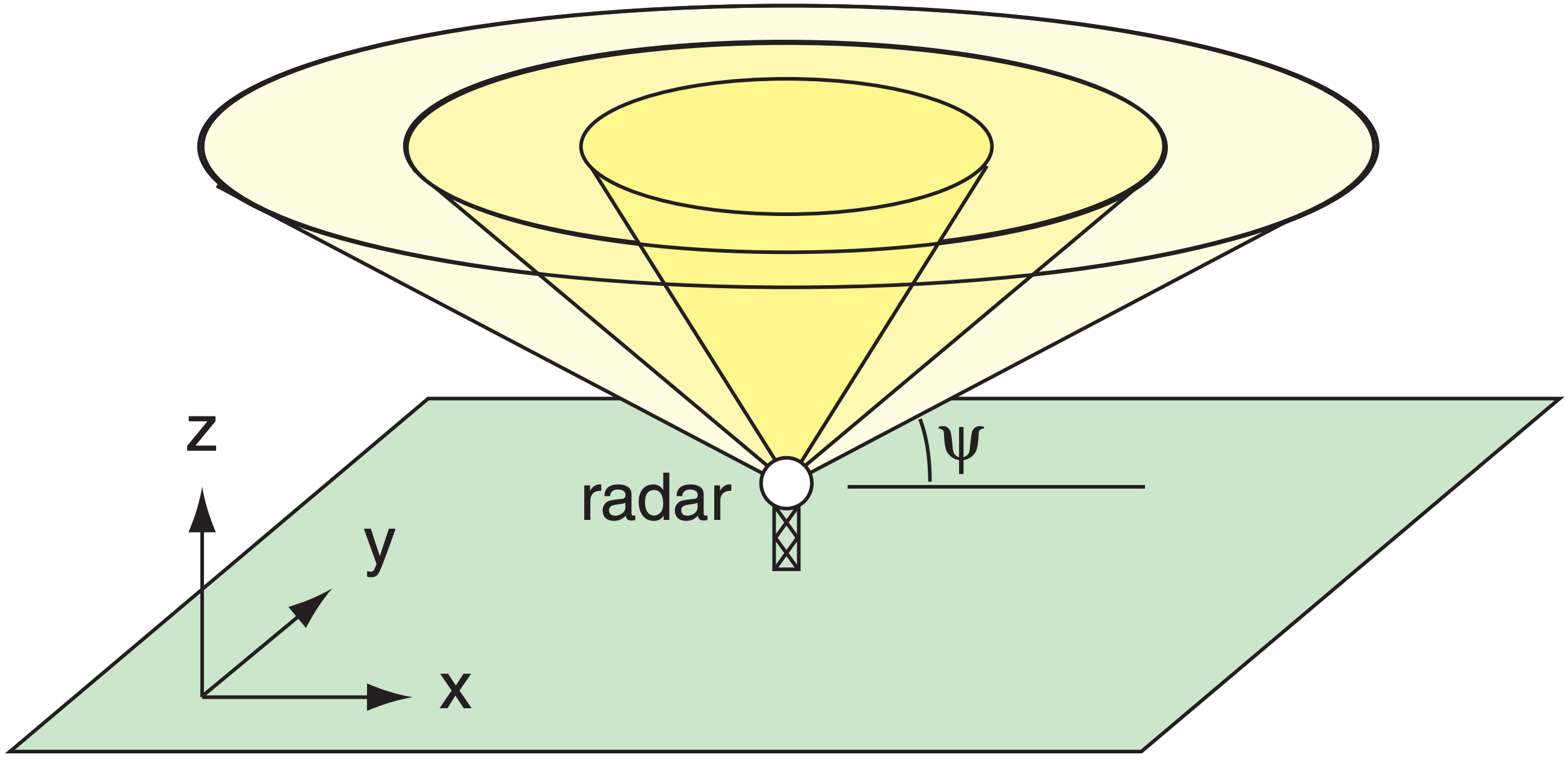
Modern weather radars are programmed to automatically sweep 360° in azimuth α, with each successive scan made at different elevation angles ψ (called scan angles). For any one elevation angle, the radar samples along the surface of a coneshaped region of air (Fig. 8.23). When all these scans are merged into one data set, the result is called a volume scan. The radar repeats these volume scans roughly every 4 to 10 minutes to sample the air around the radar.

Figure 8.23 Scan surfaces at different elevation angles ψ. For the WSR-88D, operational elevation angles range from 0.5° to 19.5°.

Data from volume scans can be digitally sliced and displayed on computer in many forms. Animations of these displays over time are called radar loops. Typical 2-D displays are:

Figure 8.24 (a) Plan-Position Indicator (PPI) display. (b) Constant Altitude Plan Position Indicator (CAPPI) display.

Figure 8.25 (a) Range Height Indicator (RHI) display. (b) Arbitrary Vertical Cross Section (AVCS) display

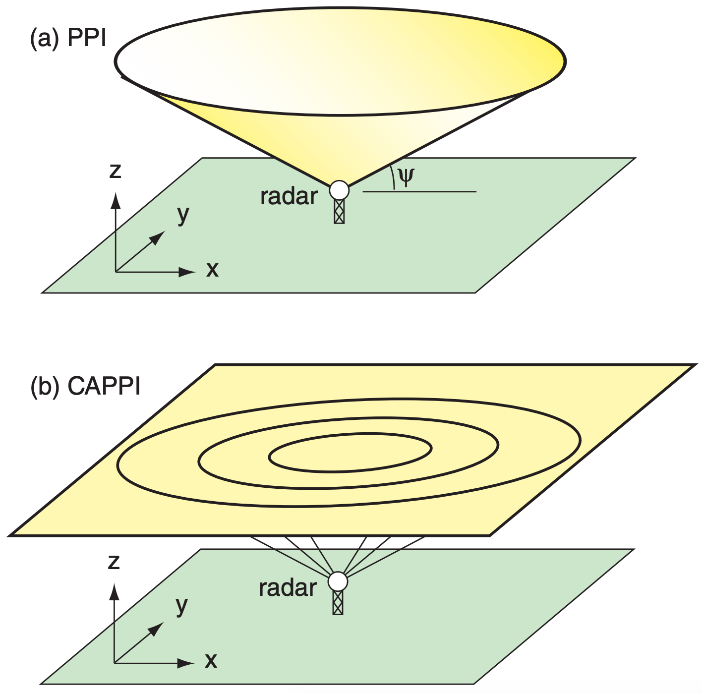
• PPI (plan position indicator), which shows the radar echoes around 360° azimuth, but at only one elevation angle. Namely, this data is from a cone that spans many altitudes (Fig. 8.24a). These displays are often superimposed on background maps showing towns, roads and shorelines.
• CAPPI (constant-altitude plan position indicator), which gives a horizontal slice at any altitude (Fig. 8.24b). These displays are also superimposed on background maps (Fig. 8.26). At long ranges, the CAPPI is often allowed to follow the PPI cone from the lowest elevationangle scan.
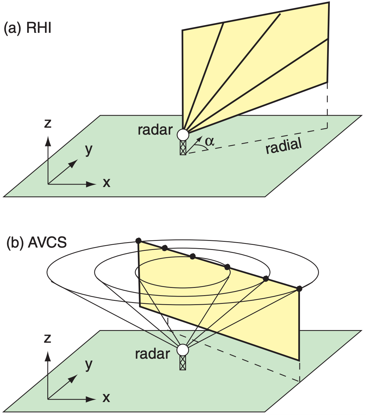
• RHI (range-height indicator, see Fig. 8.25a), which is a vertical slice along a fixed azimuth (α) line (called a radial) from the radar. It is made by physically keeping the antenna dish pointed at one azimuth while stepping the elevation angle up and down.
• AVCS (arbitrary vertical cross section), which gives a vertical slice in any horizontal direction through the atmosphere (Fig. 8.25b).

8.3.1.3. Radar Bands

In the microwave portion of the electromagnetic spectrum are wavelength (λ) bands that have been assigned for use by radar (Fig. 8.4d). Each band is given a letter designation:

• L band: λ = 15 to 30 cm. Used in air traffic control and to study clear-air turbulence (CAT).
• S band: λ = 7.5 to 15 cm. Detects precipitation particles, insects, and birds. Long range (roughly 500 km) capabilities, but requires a large (9 m diameter) antenna dish.
• C band: λ = 3.75 to 7.5 cm. Detects precipitation particles and insects. Shorter range (roughly 250 km because the microwave pulses are more quickly attenuated by the precipitation), but requires less power and a smaller antenna dish.
• X band: λ = 2.5 to 3.75 cm. Detects tiny cloud droplets, ice crystals and precipitation. Large attenuation, therefore very short range. The radar sensitivity decreases inversely with the 4^th power of range.
• K band is split into two parts:

  Ku band: λ = 1.67 to 2.5 cm

  Ka band: λ = 0.75 to 1.11 cm.

  Detects even smaller particles, but has a shorter range. (The gap at 1.11 to 1.67 cm is due to very strong absorption by a water-vapor line, causing the atmosphere to be opaque at these wavelengths; see Fig. 8.4d).

The US National Weather Service’s nationwide network of 159 NEXRAD (Next Generation Radar) Weather Surveillance Radars (WSR-88D) uses the S band (10 cm) to detect storms and estimate precipitation. The Canadian Meteorological Service is replacing their C-band (5 cm) radars with 20 S-band klystron radars. Some North American TV stations also have their own C-band weather radars. Europe is moving to a C-band standard for weather radars, although some S-band radars are also used in Spain. Weather-avoidance radars on board commercial aircraft are X band, to help alert the pilots to stormy weather ahead. Police radars include X and K bands, while microwave ovens use S band (12.2 cm). All bands are used for weather research.

Figure 8.26 CAPPI display of radar reflectivity (related to rainfall intensity) of a violent squall line of thunderstorms (orange-red curved line through center of image) sweeping across Pennsylvania in 2003. [Courtesy of the US National Weather Service.]

8.3.1.4. Beam Propagation

A factor leading to erroneous signals is ground clutter. These are undesired returns from fixed objects (tall towers, trees, buildings, mountains). Usually, ground clutter is found closest to the radar where the beam is still low enough to hit objects, although in mountainous regions ground clutter can occur at any range where the beam hits a mountain. Ground-clutter returns are often strong because these targets are large. But these targets do not move, so they can be identified as clutter and filtered out. However, swaying trees and moving traffic on a highway can confuse some ground-clutter filters.

In a vacuum, the radar pulses would propagate at the speed of light in a straight line. However, in the atmosphere, the denser and colder the air, the slower the speed. A measure of this speed reduction is the index of refraction, n:

\(\ \begin{align} n=c_{o} / c\tag{8.18}\end{align}\)

where c_o = 299,792,458 m s^–1 is the speed of electromagnetic radiation in a vacuum, and c is the speed in air. The slowdown is very small, giving index-of-refraction values on the order of 1.000325.

To focus on this small change, a new variable called the refractivity, N, is defined as

\(\ \begin{align} N=(n-1) \times 10^{6}\tag{8.19}\end{align}\)

For example, if n = 1.000325, then N = 325. For radio waves, including microwaves:

\(\ \begin{align} N=a_{1} \cdot \frac{P}{T}-a_{2} \cdot \frac{e}{T}+a_{3} \cdot \frac{e}{T^{2}}\tag{8.20}\end{align}\)

where P is atmospheric pressure at the beam location, T is air temperature (in Kelvin), e is water vapor pressure, a₁ = 776.89 K kPa^–1, a₂ = 63.938 K kPa^–1, and a₃ = 3.75463x106 K2 kPa^–1. In the first term on the RHS, P/T is proportional to air density, according to the ideal gas law. The other two terms account for the polarization of microwaves by water vapor (polarization is discussed later). The parameters in this formula have been updated to include current levels of CO₂ (order of 375 ppm) in the atmosphere.

Sample Application

Find the refractivity and speed of microwaves through air of pressure 90 kPa, temperature 10°C, and relative humidity 80%.

Find the Answer

Given: P = 90 kPa, T = 10°C = 283 K, RH = 80%

Find: N (dimensionless) and c (m·s^–1)

First, convert RH into vapor pressure. Knowing T, get the saturation vapor pressure from Table 4-1 in the Water Vapor chapter: e_s = 1.233 kPa. Then use eq. (4.14): e = RH·e_s = 0.80·(1.233 kPa). e = 0.986 kPa

Next, use P, T, and e in eq. (8.20):

N= (776.89 K/kPa)·(90kPa)/(283K) – (63.938 K/kPa)·(0.986kPa)/(283K) + (3.75463x10⁶ K²/kPa)·(0.986kPa)/(283K)²

N = 247.067 – 0.223 + 46.224 = 293.068

Solve eq. (8.18) for c, and plug in n from (8.19):

c = c_o / [1 + Nx10^–6 ] = (299,792,458 m/s) / 1.000293

c = 299,704,624.2 m s^–1

Check: Units OK. Physics OK.

Exposition: The military carefully monitors and predicts vertical profiles of refractivity to determine whether the signal from their air-defense radars would get ducted or trapped, which would prevent them from detecting enemy aircraft sneaking in above the duct.

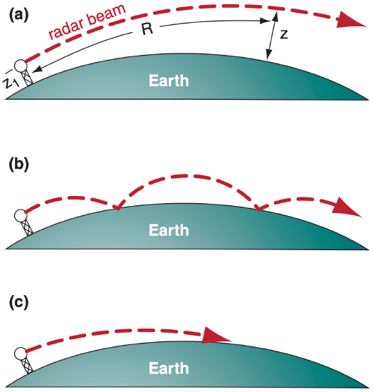
Although small, the change in propagation speed through air is significant because it causes the microwave beam to refract (bend) toward the denser, colder air. Recall from chapter 1 that density decreases nearly exponentially with height, which results in a vertical gradient of refractive index ∆n/∆z. This causes microwave beams to bend downward. But the Earth’s surface also curves downward relative to the starting location. When estimating the beam height z above the Earth’s surface at slant range R, you must include both effects.

One way to estimate this geometrically is to assume that the beam travels in a straight line, but that the Earth’s surface has an effective radius of curvature R_c of

\(\ \begin{align} R_{c}=\frac{R_{o}}{1+R_{o} \cdot(\Delta n / \Delta z)}=k_{e} \cdot R_{o}\tag{8.21}\end{align}\)

where R_o = 6371 km is the average Earth radius. The height z of the center of the radar beam can then be found from the beam propagation equation:

\(\ \begin{align} z=z_{1}-R_{c}+\sqrt{R^{2}+R_{c}^{2}+2 R \cdot R_{c} \cdot \sin \psi}\tag{8.22}\end{align}\)

knowing the height z₁ of the radar above the Earth’s surface, and the radar elevation angle ψ.

In the bottom part of the atmosphere, the vertical gradient of refractive index is roughly ∆n/∆z = –39x10^–6 km^–1 (or ∆N/∆z = –39 km^–1) in a standard atmosphere. The resulting standard refraction of the radar beam gives an effective Earth radius of approximately R_c ≈ (4/3)·R_o (Fig. 8.27a). Thus, k_e = 4/3 in eq. (8.21) for standard conditions.

Figure 8.27 (a) Standard refraction of radar beam centerline in Earth’s atmosphere. (b) Ducting or trapping over a smooth sea surface. (c) Trapping over a rough surface.

Superimposed on this first-order effect are second-order effects due to temperature and humidity variations that cause changes in refractivity gradient (Table 8-7). For example, when a cool humid boundary layer is capped by a hot dry temperature inversion, then conditions are right for a type of anomalous propagation called superrefraction. This is where the radar beam has a smaller radius of curvature than the Earth’s surface, and thus will bend down toward the Earth.

Table 8-7. Radar beam propagation conditions.
∆N/∆z (km^–1)	Refraction
> 0	subrefraction
0 to –79	normal range
–39	standard refraction
–79 to –157	superrefraction
< –157	trapping or ducting

With great enough superrefraction, the beam hits the ground and is absorbed and/or causes a ground-clutter return at that range if the Earth’s surface is rough there (Fig. 8.27c). However, for smooth regions of the Earth’s surface such as a waveless ocean, the beam can “bounce” repeatedly, which is called ducting or trapping (Fig. 8.27b).

When cooler, moister air overlies warmer drier air, then subrefraction occurs, where the radius of curvature is larger than for standard refraction. This effect is limited by the fact that atmospheric lapse rate is rarely statically unstable over large depths of the mid and upper troposphere.

Sample Application(§)

For a radar on a 10 m tower, plot the centerline height (relative to the Earth’s surface) of the beam vs. range for standard refraction, for a 1° elevation angle.

Find the Answer

Given: ∆N/∆z = –39 km^–1, z₁ = 10 m = 0.01 km, R_o = 6371 km

Find: z (km) vs. R (km)

∆N/∆z = –39 km^–1. Thus ∆n/∆z = –39x10^–6 km^–1 .

Use eq. (8.21):

R_c = (6371 km) / [1+(6356.766 km)(–39x10^–6 km^–1)] = (6371 km) · 1.33 = 8473 km

Use eq. (8.22): z = 0.01 km – 8473 km + [ R² +(8473 km)² + 2·R·(8473 km)·sin(1°) ]^1/2

For example, z = 2.35 km at R = 100 km. Using a spreadsheet for many different R values gives:

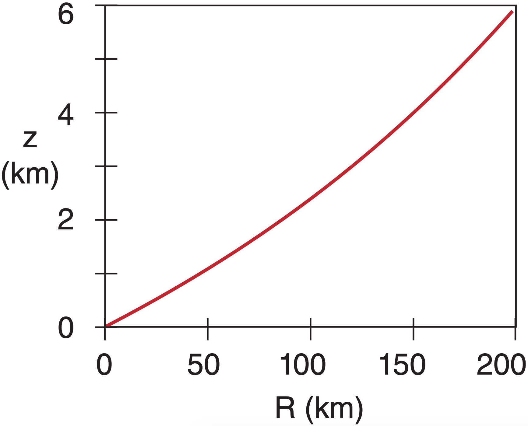
Check: Units OK. Physics OK. Graph reasonable.

Exposition: Why does the line curve up with increasing range? Although the radar beam bends downward, the Earth’s surface curves downward faster.

8.3.2. Reflectivity

8.3.2.1. The Radar Equation

Recall that the radar transmits an intense pulse of microwave energy with power P_T (≈ 750 kW for WSR-88D radars). Particles in the atmosphere scatter a minuscule amount of this energy back to the radar, resulting in a small received power P_R. The ratio of received to transmitted power is explained by the radar equation:

\(\begin{align} \left [\frac{P_{R}}{P_{T}}\right]=\quad[b] \quad\quad\cdot\quad\left[\frac{|K|}{L_{a}}\right]^{2} \quad\cdot\quad\left[\frac{R_{1}}{R}\right]^{2} \quad\quad\cdot\quad\left[\frac{Z}{Z_{1}}\right]\tag{8.23}\end{align}\)
\(\left[\begin{array}{l}{\text {relative}} \\ {\text {received}} \\ {\text {power}}\end{array}\right]=\left[\begin{array}{l}{\text {equip-}} \\ {\text { ment }} \\ {\text { effects }}\end{array}\right] \cdot\left[\begin{array}{l}{\text {atmos}-} \\ {\text { pheric }} \\ {\text { effects }}\end{array}\right] \cdot\left[\begin{array}{l}{\text { range }} \\ {\text { inverse }} \\ {\text { squared }}\end{array}\right]\cdot\left[\begin{array}{l}{\text { target }} \\ {\text { refect }-} \\ {\text { ivity }}\end{array}\right]\)

where each factor in brackets is dimensionless.

The most important parts of this equation are the refractive-index magnitude |K|, the range R between the radar and target, and the reflectivity factor Z. These are summarized below. The Info Box has more details on the radar equation.

|K| (dimensionless): Liquid drops are more efficient at scattering microwaves than ice crystals.

|K|² ≈ 0.93 for liquid drops, and |K|² ≈ 0.208 for ice (assuming spherical ice particles of the same mass as the actual snow crystal).

R (km): Returned energy from more distant targets is weaker than from closer targets, as given by the inverse-square law (see Radiation chapter).

Z (mm⁶ m^–3): Larger numbers (N) of largerdiameter (D) drops in a given volume (Vol) of air will scatter more microwave energy. This reflectivity factor is given by:

\(\ \begin{align} Z=\frac{\sum^{N} D^{6}}{V o l}\tag{8.24}\end{align}\)

where the sum is over all N drops, and where each drop could have a different D.

INFO • Deriving the Radar Equation

The radar transmits a burst of power P_T (W). As this pulse travels range R to a target drop, the energy flux (W m^–2) diminishes as it spreads to cover spherical surface area 4πR², according to the inverse square law (see the Radiation chapter). But the parabolic antenna dish focuses the energy, resulting in antenna gain G relative to the normal spherical spread of energy. While propagating to the drop, some of the energy is lost along the way, as described by attenuation factor L_a. The net energy flux E_i (W m^–2) reaching the drop is

\(\ \begin{align} E_{i}=P_{T} \cdot G /\left(4 \pi R^{2} \cdot L_{a}\right)\tag{R1}\end{align}\)

If that incident “power per unit area” hits a drop that has backscatter cross-sectional area σ, then power P_BS (W) gets scattered in all directions:

\(\ \begin{align} P_{B S}=E_{i} \cdot \sigma\tag{R2}\end{align}\)

This minuscule burst of return power spreads to cover a spherical surface area, and is again attenuated by L_a while en route distance R back to the radar. The returning energy flux E_R (W m^–2) at the radar is

\(\ \begin{align} E_{R}=P_{B S} /\left(4 \pi R^{2} \cdot L_{a}\right)\tag{R3}\end{align}\)

Eq. (R3) is similar to (R1), except that the drop does not focus the energy, so there is no gain G.

But when this flux is captured by the antenna with area A_ant and focused with gain G onto a detector, the resulting received power per drop P_R’ (W) is

\(\ \begin{align} P_{R}^{\prime}=E_{R} \cdot A_{a n t} \cdot G\tag{R4}\end{align}\)

The effective antenna area depends on many complex antenna factors, but the net result is:

\(\ \begin{align} A_{a n t}=\lambda^{2} /[8 \pi \cdot \ln (2)]\tag{R5}\end{align}\)

The radar sample volume is much larger than a single drop, thus the total returned power P_R is the sum over N drops:

\(\ \begin{align} P_{R}=\sum^{N} P_{R}\tag{R6}\end{align}\)

These N drops are contained in the sample volume Vol of air (Fig. 8.22). Assuming a cylindrical shape of length ∆R (eq. 8.14) and diameter ∆D, (eq. 8.15) gives

\(\ \begin{align} V o l=\pi R^{2} \cdot(\Delta \beta)^{2} \cdot c \cdot \Delta t / 8\tag{R7}\end{align}\)

where ∆β is beam width (radians), c is microwave speed through air, and ∆t is the radar pulse duration.

For hydrometeor particle diameters D less than a third of the radar wavelength λ, the backscatter cross-section area σ is well approximated by a relationship known as Rayleigh scattering:

\(\ \begin{align} \sigma=\pi^{5} \cdot|K|^{2} \cdot D^{6} / \lambda^{4}\tag{R8}\end{align}\)

where |K| is the refractive index magnitude of the drop or ice particle.

Combining these 8 equations, and using eq. (8.24) to define the reflectivity factor Z gives the traditional form of the radar equation:

\(\ \begin{align} P_{R}=\left[\frac{c \cdot \pi^{3}}{1024 \cdot \ln (2)}\right] \cdot\left[\frac{P_{T} \cdot G^{2} \cdot(\Delta \beta)^{2} \cdot \Delta t}{\lambda^{2}}\right] \cdot\left[\left(\frac{|K|}{L_{a} \cdot R}\right)^{2} \cdot Z\right]\tag{R9}\end{align}\)
\(P_{R}=[\text { constant }] \cdot[\text {radar characteristics}] \cdot[\text {atmos} . \text {char.}]\)

When the right side is multiplied by Z₁/Z₁ and rearranged into dimensionless groups, the result is the version of the radar equation shown as eq. (8.23).

The other factors in the radar equation are as follows:

Z₁ = 1 mm⁶ m^–3 is the reflectivity unit factor.

\(\ \begin{align} R_{1}=\operatorname{sqrt}\left(Z_{1} \cdot c \cdot \Delta t / \lambda^{2}\right)\tag{8.25}\end{align}\)

is a range factor (km), where c ≈ 3x10⁸ m s^–1 is microwave speed through air. For WSR-88D radar, wavelength λ = 10 cm and pulse duration is ∆t ≈ 1.57 µs, giving R₁ ≈ 2.17x10^–10 km.

L_a is a dimensionless atmospheric attenuation factor (L_a ≥ 1) accounting for one-way losses by absorption and scattering as the microwave pulse travels between the radar and the target drop. L_a = 1 means no attenuation, and increasing values of L_a imply increasing attenuation. For example, the signal returning from a distant rain shower is diminished (appears weaker than it actually is) if it travels through a nearby shower en route to the radar. If you don’t know L_a, then assume L_a ≈ 1.

\(\ \begin{align} b=\pi^{3} \cdot G^{2} \cdot(\Delta \beta)^{2} /[1024 \cdot \ln (2)]\tag{8.26}\end{align}\)

is a dimensionless equipment factor. For WSR-88D, the antenna gain is G ≈ 45.5 dB = 35,481 (dimensionless), and the beam width is ∆β ≈ 0.95° = 0.0161 radians, giving b ≈ 14,255.

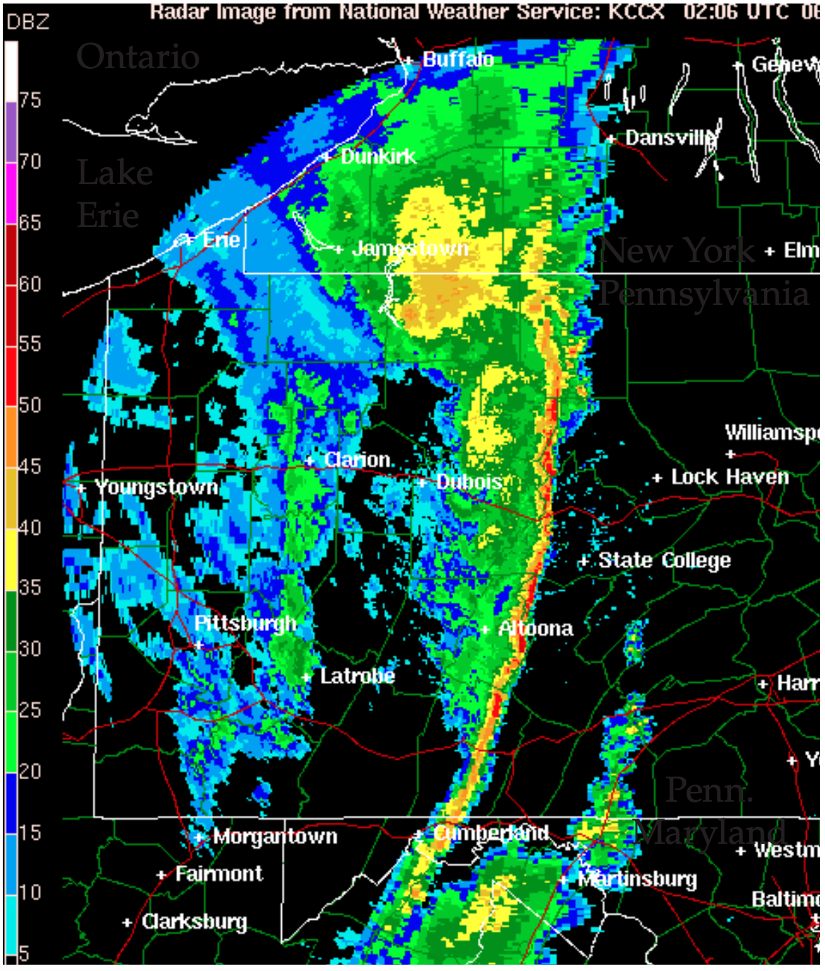
Of most interest to meteorologists is the reflectivity factor Z, because a larger Z is usually associated with heavier precipitation. Z varies over a wide range of magnitudes, so decibels (dB) of Z (namely, dBZ) are often used to quantify radar reflectivity:

\(\ \begin{align} \mathrm{dBZ}=10 \cdot \log \left(Z / Z_{1}\right)\tag{8.27}\end{align}\)

where this is a common logarithm (base 10). Although dBZ is dimensionless, the suffix “dBZ” is added after the number (e.g., 35 dBZ).

dBZ can be calculated from radar measurements of P_R/P_T by using the log form of the radar eq.:

\(\ \begin{align} d B Z=10\left[\log \left(\frac{P_{R}}{P_{T}}\right)+2 \log \left(\frac{R}{R_{1}}\right)-2 \log \left|\frac{K}{L_{a}}\right|-\log (b)\right]\tag{8.28}\end{align}\)

Although the R/R₁ term compensates for most of the decrease of echo strength with distance, atmospheric attenuation L_a still increases with range. Thus dBZ still decreases slightly with increasing range.

Reflectivity or echo intensity is the term used by meteorologists for dBZ, and this is what is displayed in radar reflectivity images. Typical values are –28 dBZ for haze, –12 dBZ for insects in clear air, 25 to 30 dBZ in dry snow or light rain, 40 to 50 dBZ in heavy rain, and up to 75 dBZ for giant hail.

Sample Application

For a 5 cm radar, the energy scattered from a 1 mm diameter drop is how much greater than that from a 0.5 mm drop?

Find the Answer

Given: λ = 5 cm, D1 = 0.5 mm, D2 = 1 mm

Find: σ_scat2 / σ_scat1 (dimensionless)

For Rayleigh scattering [see Info Box eq. (R8)]:

σ_scat2 / σ_scat1 = (D₂/D₁)⁶ = 2⁶ = 64 .

Check: Units OK. Physics OK.

Exposition: Amazingly large difference. Double the drop size and get 64 times the scattered energy.

Sample Application

WSR-88D radar detects a 40 dBZ rain shower 20 km from the radar, with no other rain detected. Transmitted power was 750 kW, what is the received power?

Find the Answer

Given: Echo = 40 dBZ, R = 20 km, P_T = 750,000 W, |K|² = 0.93 for rain (i.e., liquid), b = 14,255 , R₁ = 2.17x10^–10 km for WSR-88D.

Find: P_R = ? W

Assume: L_a = 1.0 (no attenuation), because there are no other rain showers between the radar and target.

Use eq. (8.27) and rearrange to solve for Z/Z₁ : Z/Z₁ = 10^(dBZ/10) = 10^(40/10) = 10⁴.

Use the radar equation (8.23): P_R = (7.5x10⁵W)·(14,255)·(0.93)·[(2.17x10^–10km)/(20km)]²}·[10⁴]

P_R = 1.17 x 10^–8 W .

Check: Units OK. Physics OK.

Exposition: With so little power coming back to the radar, very sensitive detectors are needed. WSR-88D radars can detect signals as weak as P_R ≈ 10^–15 W.

Normal weather radars use the same parabolic antenna dish to receive signals as to transmit. But such an intense pulse is transmitted that the radar antenna electrically “rings” after the transmit impact for 1 µs, where this “ringing” sends strong power as a false signal back toward the receiver. To compensate, the radar must filter out any received energy during the first 1 µs before it is ready to detect the weak returning echoes from true meteorological targets. For this reason, the radar cannot detect meteorological echoes within the first 300 m or so of the radar.

Even when looking at the same sample volume of rain-filled air, the returned power varies considerably from pulse to pulse. To reduce this noise, the WSR-88D equipment averages about 25 sequential pulses together to calculate each smoothed reflectivity value that is shown on the radar display for each sample volume.

8.3.2.2. Rainfall Rate from Radar Reflectivity

A tenuous, but useful, relationship exists between rainfall rate and radar echo intensity. Both increase with the number and size of drops in the air. However, this relationship is not exact. Complicating factors on the rainfall rate RR include the drop terminal velocity, partial evaporation of the drops while falling, and downburst speed of the air containing the drops. Complicating factors for the echo intensity include the bright-band effect (see next page), and unknown backscatter cross sections for complex ice-crystal shapes.

Nonetheless, an empirically tuned approximation can be found:

\(\ \begin{align} R R=a_{1} \cdot 10^{\left(a_{2} \cdot d B Z\right)}\tag{8.29}\end{align}\)

where a₁ = 0.017 mm h^–1 and a₂ = 0.0714 dBZ^–1 (both a₂ and dBZ are dimensionless) are the values for the USA WSR-88D radars. This same equation can be written as:

\(\ \begin{align} Z=a_{3} \cdot R R^{a_{4}}\tag{8.30}\end{align}\)

where a₃ = 300, and a₄ = 1.4, for RR in mm h^–1 and Z in mm⁶ m^–3. Equations such as (8.29) and (8.30) are called Z-R relationships.

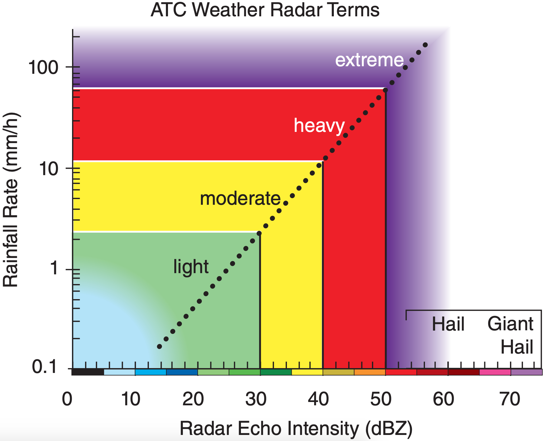
To simplify storm information presented to the public, radar reflectivities are sometimes binned into categories or levels with names or numbers representing rainfall intensities. For example, aircraft pilots and controllers use the terms in Fig. 8.28. TV weathercasters often display the intensity categories in different colors. Different agencies in different countries use different thresholds for precipitation categories. For example, in Canada moderate precipitation is defined as 2.5 to 7.5 mm h^–1.

Figure 8.28 Precipitation-intensity terms as a function of weather-radar echo reflectivity, as used by the USA Air Traffic Control (ATC). Rainfall rate is approximate, based on eq. (8.29). For any dBZ on the horizontal axis, conceptually draw a vertical line up to the dotted line, and then look horizontally to the left to estimate the precipitation rate.

Z-R relationships can never be perfect, as is demonstrated here. Within an air parcel of mass 1 kg, suppose that m_L = 5 g of water has condensed and falls out as rain. If that 5 g is distributed equally among N = 1000 drops, then the diameter D of each drop is 2.12 mm, from:

\(\ \begin{align} D=\left[\frac{6 \cdot m_{L}}{\pi \cdot N \cdot \rho_{l i q}}\right]^{1 / 3}\tag{8.31}\end{align}\)

where ρ_liq = 10³ kg m^–3 is the density of liquid water. However, if the same mass of water is distributed among N = 10,000 droplets, then D = 0.98 mm. When these two sets of N and D values are used in eq. (8.24), the first scenario gives 10 times the reflectivity Z as the second, even though they have identical total mass of liquid water m_L and identical rainfall amount. Nonetheless, Z-R relationships are useful at giving a first approximation to rainfall rate.

Sample Application

If radar reflectivity is 35, what is the ATC precipitation intensity term? Also, estimate the rainfall rate.

Find the Answer

Given: reflectivity = 35 dBZ

Find: ATC term and RR = ? mm h^–1.

Use Fig. 8.28: ATC weather radar term = moderate.

Use eq. (8.29):

RR = (0.017mm h^–1)·10^{[0.0714(1/dBZ)·35dBZ]} = 5 mm h^–1.

Check: Units OK. Physics OK.

Exposition: Heavy and extreme echoes are often associated with thunderstorms, which pilots avoid.

Sample Application

Air parcels A and B both have liquid-water mixing ratio 3 g kg^–1, but A has 1000 active liquid-water nuclei and B has 5,000. Compare the dBZ from both parcels.

Find the Answer

Given: r_L = 3 g kg^–1, ρ_L = 10³ kg m^–3, N_A = 1000 , N_B = 5000 .

Find: dBZ_A and dBZ_B (dimensionless)

Assume air density is ρ = 1 kg/m³. Assume Vol.=1 m³

Assume equal size droplets form on each nucleus, so that ΣD⁶ = N·D⁶.

Use eq. (8.31):

DA=[6·(0.003kg)/(π·1000·(10³ kg m^–3)]^1/3 = 0.00179 m = 1.79 mm

DB=[6·(0.003kg)/(π·5000·(10³ kg m^–3)]^1/3 = 0.00105 m = 1.05 mm

Use eq. (8.24), but using N·D⁶ in the numerator:

Z_A = 1000·(1.79 mm)⁶ /(1 m³) = 3.29x10⁴ mm6 m^–3

Z_B = 5000·(1.05 mm)⁶ /(1 m³) = 6.70x10³ mm6 m^–3

Use eq. (8.27):

dBZ_A = 10·log[ (3.29x10⁴ mm⁶ m^–3)/(1 mm⁶ m^–3) ] = 45.2 dBZ

dBZ_B = 10·log[ (6.70x10³ mm⁶ m^–3)/(1 mm⁶ m^–3) ] = 38.3 dBZ

Check: Units OK. Physics OK.

Exposition: Thus, the same amount of liquid water (3 g kg^–1) in each parcel would lead to substantially different radar reflectivities. This is the difficulty of Z-R relationships. But not all is lost -- the polarization radar section shows how more accurate rainfall estimates can be made using radar

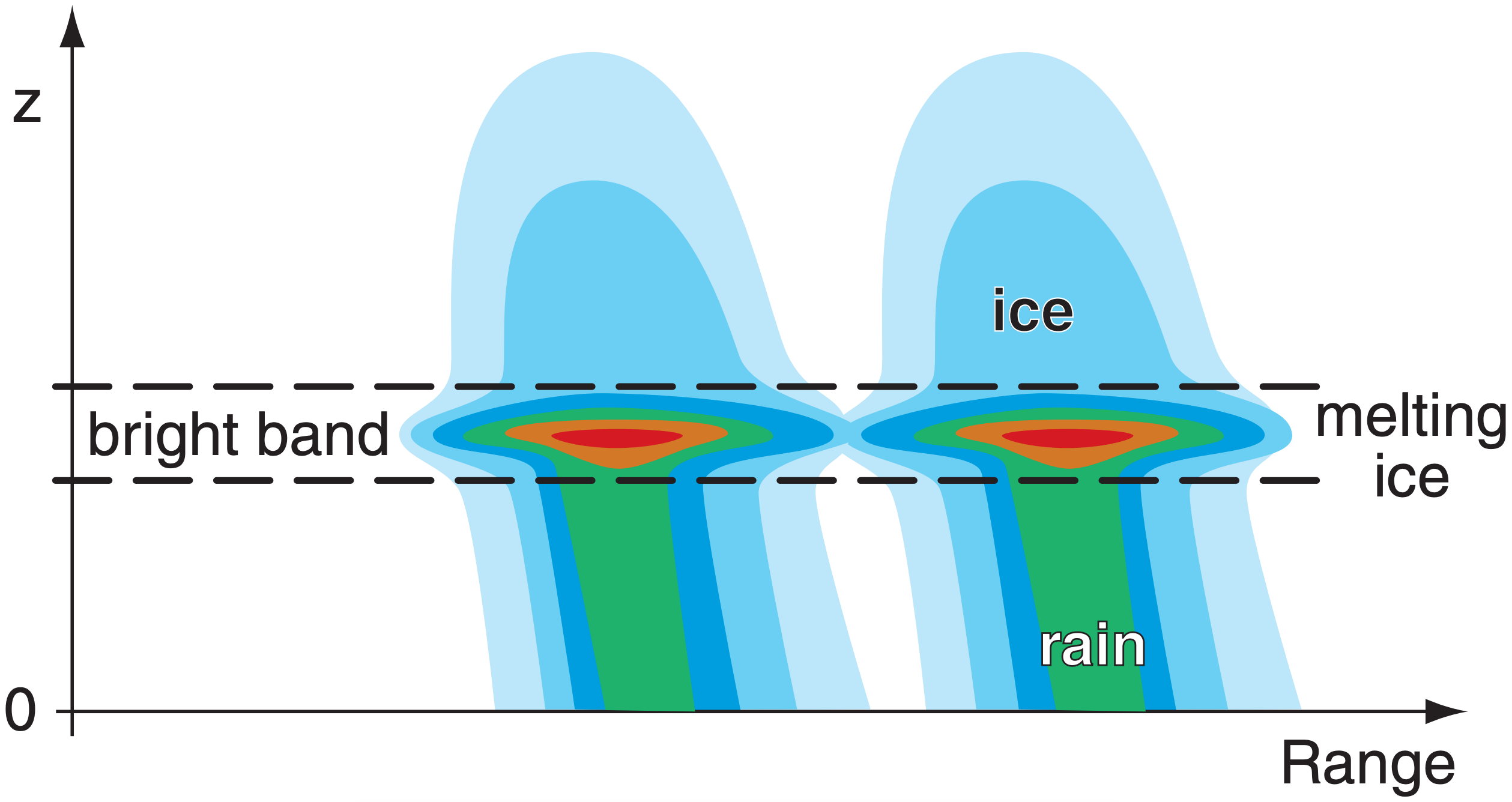
8.3.2.3. Bright Band

Ice crystals scatter back to the radar only about 20% of the energy scattered by the same amount of liquid water (as previously indicated with the |K|² factor in the radar equation). However, when ice crystals fall into a region of warmer air, they start to melt, causing the solid crystal to be coated with a thin layer of water. This increases the reflectivity of the liquid-water-coated ice crystals by a factor of 5, causing a very strong radar return known as the bright band. Also, the wet outer coating on the ice crystals cause them to stick together if they collide, resulting in a smaller number of larger-diameter snowflake clusters that contribute to even stronger returns.

As the ice crystals continue to fall and completely melt into liquid drops, their diameter decreases and their fall speed increases, causing their drop density and resulting reflectivity to decrease. The net result is that the bright band is a layer of strong reflectivity at the melting level of falling precipitation. The reflectivity in the bright band is often 15 to 30 times greater than the reflectivity in the ice layer above it, and 4 to 9 times greater than the rain layer below it. Thus, Z-R relationships fail in bright-band regions.

In an RHI display of reflectivity (Fig. 8.29), the bright band appears as a layer of stronger returns. In a PPI display the bright band is donut shaped — a hollow circle of stronger returns around the radar, with weaker returns inside and outside the circle.

Figure 8.29 RHI sketch of the bright band in two precipitation cells. Colors mimic radar dBZ.

8.3.2.4. Hail

Hail can have exceptionally high radar reflectivities, of order 60 to 75 dBZ, compared to typical maxima of 50 dBZ for heavy rain. Because hailstone size is too large for microwave Rayleigh scattering to apply, the normal Z-R relationships fail. Some radar algorithms diagnose hail for reflectivities > 40 dBZ at altitudes where the air is colder than freezing, with greater chance of hail for reflectivities ≥ 50 dBZ at altitudes where temperature ≤ –20°C.

8.3.2.5. Other Uses for Reflectivity Data

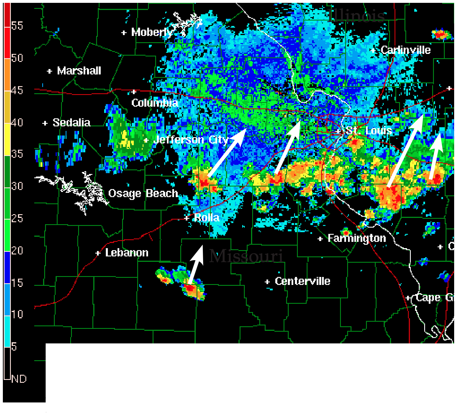
Radar reflectivity images are used by meteorologists to identify storms (thunderstorms, hurricanes, mid-latitude cyclones), track storm movement, find the height of thunderstorm features such as the top of the radar-echo (echo-top height), indicate likelihood of hail, and estimate rain rate and flooding potential. For example, Fig. 8.30 shows isolated thunderstorm cells, while Fig. 8.26 shows an organized squall line of thunderstorms. The radar image typically presented by TV weather briefers is the reflectivity image.

Figure 8.30 CAPPI image of thunderstorm cells (orange & red), near St. Louis, MO, on 22 July 2004. White vectors indicate cell movement. (Courtesy of the US NWS.)

Clear-air reflectivities from bugs can help identify cold fronts, dry lines, thunderstorm outflow (gust fronts), sea-breeze fronts, and other boundaries (discussed later in this book). Weather radar can also track bird migration. Clear-air returns are often very weak, so radar clear-air scan strategies use a slower azimuth sweep rate and longer pulse duration to allow more of the microwave energy to hit the target and to be scattered back to the receiver.

8.3.3. Doppler Radar

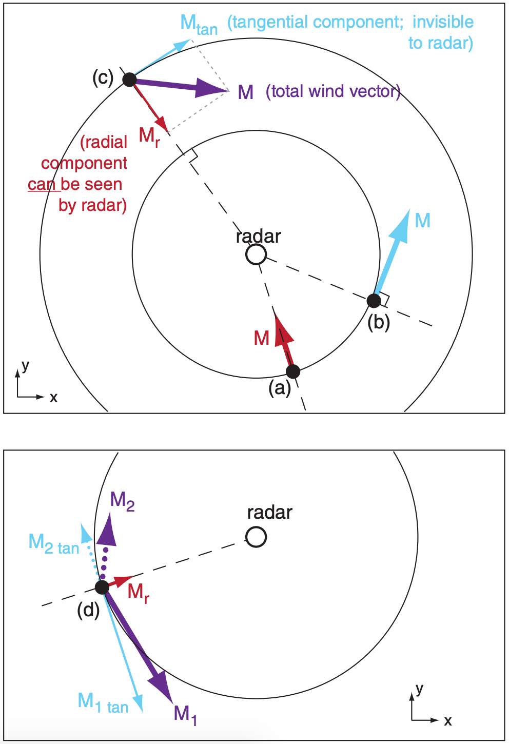
Large hydrometeors include rain drops, ice crystals, and hailstones. Hydrometeor velocity is the vector sum of their fall velocity through the air plus the air velocity itself. Doppler radars measure the component of hydrometeor velocity that is away from or toward the radar (i.e., radial velocity, Fig. 8.31). Hence, Doppler radars can detect wind components associated with gust fronts and tornadoes.

Figure 8.31 Illustration of which velocities can be seen by Doppler radar. For any location where you know the wind vector, mentally draw a circle (centered on the radar) that passes through the location, and draw a radial line (shown dashed in these figures) from the radar to the location. The radar can see only the component of the wind vector along the radial line, and cannot see the component along the circle. Examples: At point (a) the total wind vector M is along the radial line, hence the radar sees the whole wind. At point (b) the total wind vector M is tangent to the circle, hence the radar sees zero wind there. At point (c) the total wind vector M has a radial component M_r that the radar sees, and a tangential component M_tan that is invisible. Hence, only a portion of the total wind is seen there.

Conversely, if you don’t know the actual wind but have Doppler radar observations, beware that an infinite number of true wind vectors can create the radial component seen by the radar. For example, at point (d) two completely different wind vectors M₁ and M₂ have the same radial component M_r. Hence, the radar would give you only M_r but you would have no way of knowing the total wind vector.

The solution to this dilemma is to have two Doppler radars (i.e., dual Doppler) at different locations that can both scan the same wind location from different directions. The WSR-88D radar network in the USA is programmed to provide dual Doppler information.

8.3.3.1. Radial Velocities

Radars transmit a microwave signal of known frequency ν. But once scattered from moving hydrometeors, the microwaves that return to the radar have a different frequency ν + ∆ν. Hydrometeors moving toward the radar cause higher returned frequencies while those moving away cause lower frequencies. The frequency change ∆ν is called the Doppler shift.

Doppler-shift magnitude can be found from the Doppler equation:

\(\ \begin{align} |\Delta v|=\frac{2 \cdot\left|M_{r}\right|}{\lambda}\tag{8.32}\end{align}\)

where λ is the wavelength (e.g., S-band radars such as WSR-88D use λ = 10 cm), and M_r is the average radial velocity of the hydrometeors relative to the radar. Knowing the speed of light c = 3x10⁸ m s^–1, you can find the frequency as a function of wavelength:

\(\ \begin{align} v=c / \lambda\tag{8.33}\end{align}\)

However, the frequency shift is so minuscule that it is very difficult to measure (see Sample Application).

Sample Application

An S-band radar would measure what Dopplershift magnitude for a tornadic speed of 90 m s^–1?

Find the Answer

Given: M_r = 90 m/s, assume λ = 10 cm for S-band.

Find: ∆ν = ? s^–1

Use eq. (8.32): |∆ν| = [2·(90 m s^–1)] / ( 0.1 m) = 1800 s^–1

Check: Units & physics OK.

Exposition: The Doppler-shift magnitude is less than one part per million, relative to the original transmitted frequency (eq. 8.33) of ν = c/λ = (3x10⁸ m s^–1) / (0.1 m) = 3x10⁹ s^–1.

Instead, Doppler radars detect air motion by measuring the phase shift of the microwaves. Consider a pulse of microwaves that scatter from a droplet-laden air parcel (Fig. 8.32). When that parcel is at any one location and is illuminated by a radar pulse, there can be a measurable phase difference (difference in locations of the wave troughs) between the incident wave and the scattered wave. Fig. 8.33a illustrates a phase difference of zero; namely, the troughs coincide.

Figure 8.32 A pulse of microwaves scatters off a stationary, droplet-laden air parcel that coincides with the radar sample volume. The same shading (solid for incident pulse, dashed for reflected pulse) is used in the next two figures.

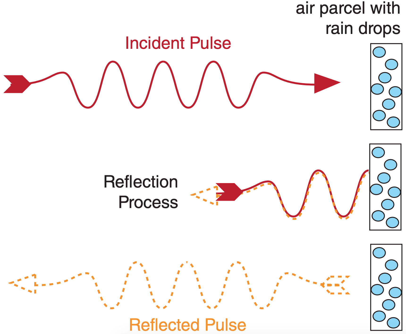
If the parcel has moved to a slightly different distance from the radar when the next pulse hits, then there will be a different phase shift compared to that of the first pulse (Fig. 8.33b). As illustrated, the phase shift ∆d is twice the radial distance ∆R that the air parcel moved. You can demonstrate this to yourself by drawing a perfect wave on a thin sheet of tracing paper, folding the paper horizontally a certain distance ∆R from the crest, and then comparing the distance ∆d between incident and folded troughs or crests. Knowing the time between successive pulses (= 1/PRF), the radial velocity M_r is:

\(\ \begin{align} M_{\mathrm{r}}=\Delta R \cdot \mathrm{PRF}=\mathrm{PRF} \cdot \Delta d / 2\tag{8.34}\end{align}\)

Figure 8.33 Phase shift distance is twice the distance moved by the air parcel.

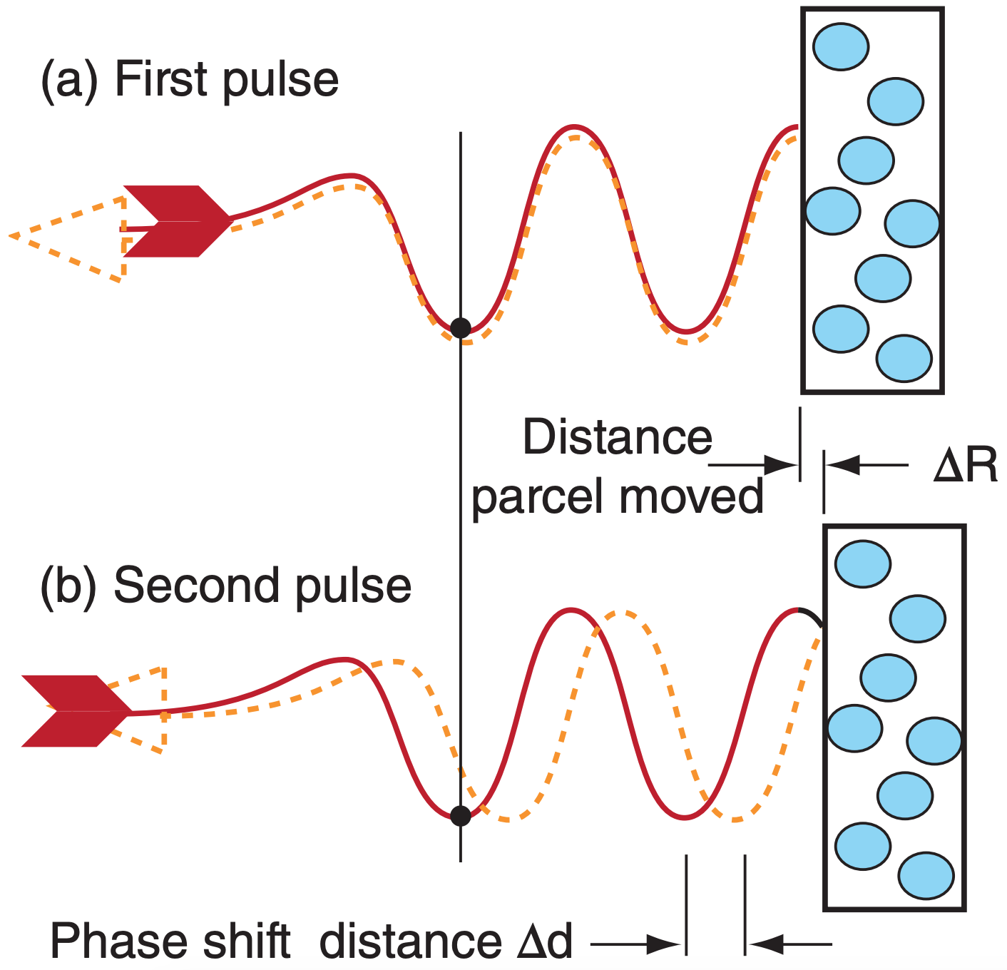
Table 8-8 gives the display convention for PPI or CAPPI displays of Doppler radial velocities in North America. Faster speeds are sometimes displayed with brighter lighter colors. The color convention is modeled after the astronomical “red shift” for stars moving away from Earth. In directions from the radar that are perpendicular to the mean wind, there is no radial component of wind (Fig. 8.31); hence, this appears as a white or light grey line (Fig. 8.38a) of zero radial velocity (called the zero isodop). In some countries, the zero isodop is displayed with finite width as a black “no-data” line, because the ground-clutter filter eliminates the slowest radial velocities.

Table 8-8. Display convention for Doppler velocities.
Sign of Mr	Radial Direction Relative to Radar	Display Color
Positive	AWAY	Red & Orange
Zero	(none)	White, Grey or Black
Negative	TOWARD	Green & Blue

8.3.3.2. Maximum Unambiguous Velocity

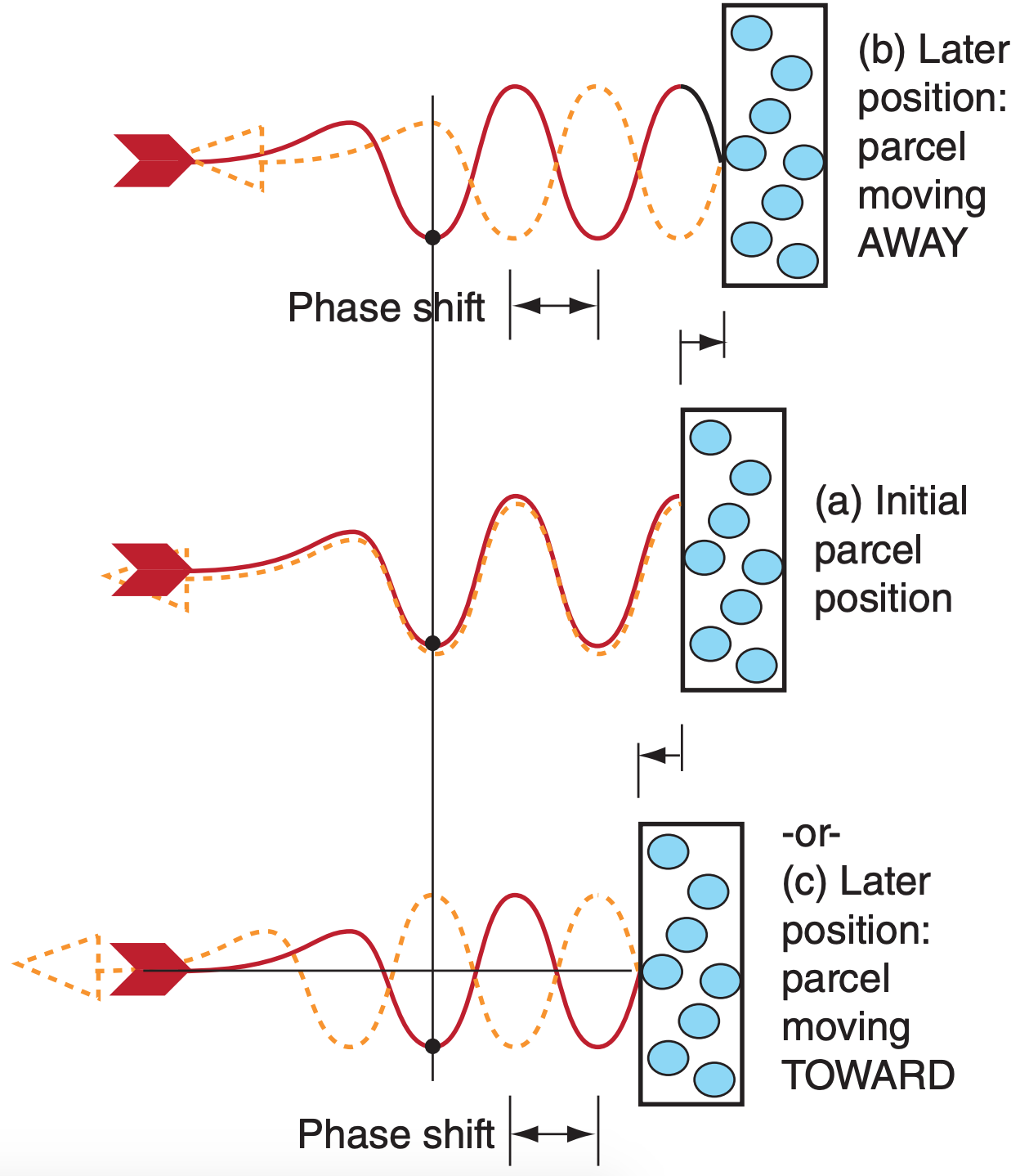
The phase-shift method imposes a maximum unambiguous velocity M_{r max} the radar can measure, given by:

\(\ \begin{align} M_{\mathrm{r} \max }=\lambda \cdot \mathrm{PRF} / 4\tag{8.35}\end{align}\)

where λ is wavelength. Fig. 8.34 shows the reason for this limitation. From the initial pulse to the second pulse, if the air parcel moved a quarter wavelength (λ/4) AWAY from the radar (Fig. 8.34b), then the scattered wave is a half wavelength out of phase from the incident wave. However, if the air parcel moved a quarter wavelength TOWARD the radar (Fig. 8.34c), then the phase shift is also half a wave length. Namely, the AWAY and TOWARD velocities give exactly the same phase-shift signal at this critical speed, and the radar phase detector cannot distinguish between them.

Figure 8.34 An air-movement distance of one quarter a wavelength toward or away from the radar can yield identical phase shifts, making velocity interpretation ambiguous (i.e., erroneous).

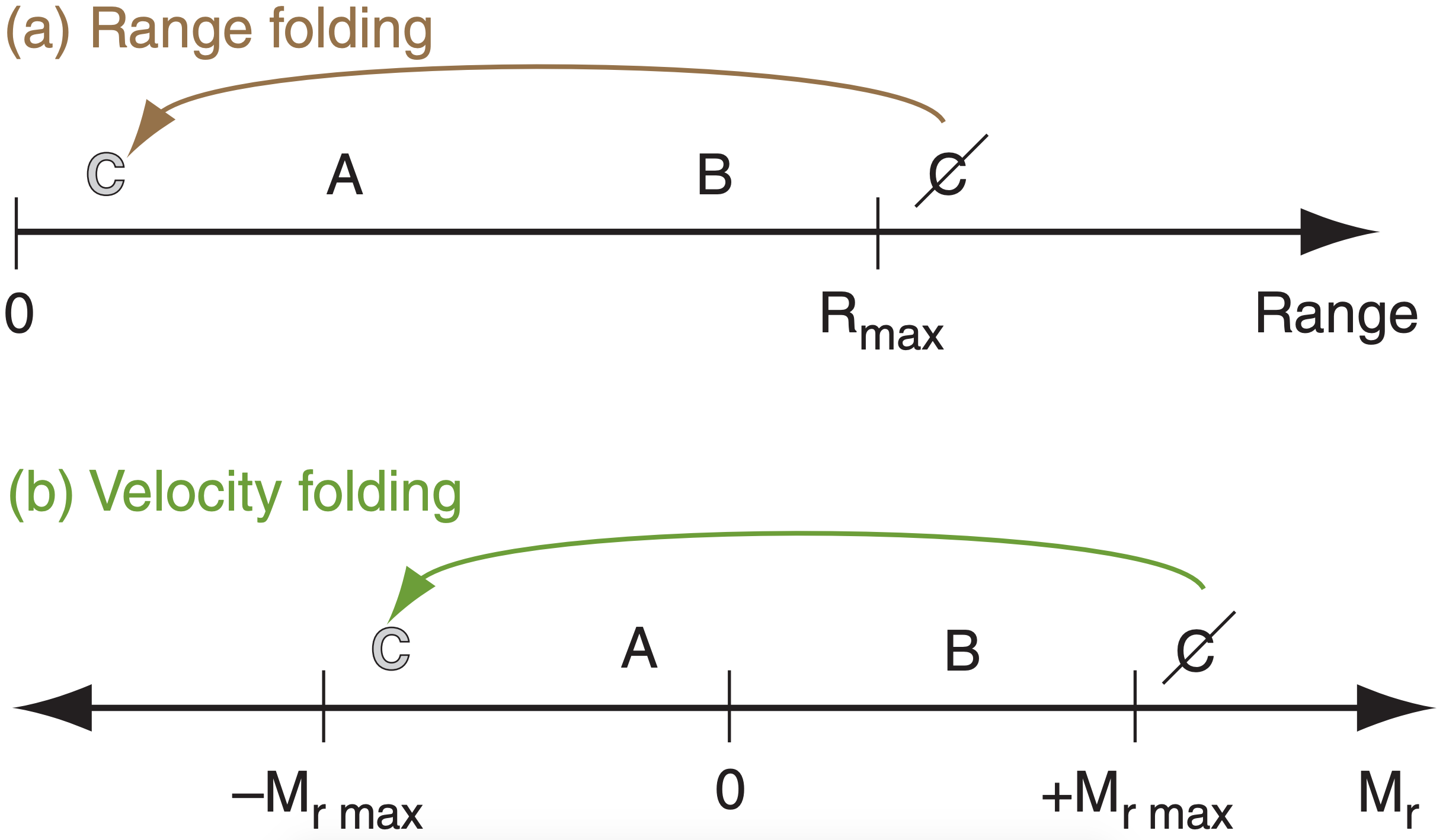
Velocities slightly faster than M_{r max} AWAY from the radar erroneously appear to the phase detector as fast velocities TOWARD the radar. Similarly, velocities faster than M_{r max} TOWARD the radar are erroneously folded back as fast AWAY velocities. The false, displayed velocities M_{r false} are:

For M_{r max} < M_r < 2M_{r max} :

\(\ \begin{align} M_{\mathrm{r} \text { false }}=M_{\mathrm{r}}-2 M_{\mathrm{r} \max }\tag{8.36a}\end{align}\)

For (– 2M_{r max}) < M_r < (–M_{r max}) :

\(\ \begin{align} M_{\mathrm{r} \text { false }}=M_{\mathrm{r}}+2 M_{\mathrm{r} \max }\tag{8.36b}\end{align}\)

Speeds greater than 2|M_{r max}| fold twice.

For greater max velocities M_{r max} , you must operate the Doppler radar at greater PRF (see eq. 8.35). However, to observe storms at greater range Rmax, you need lower PRF (see eq. 8.17). This trade-off is called the Doppler dilemma (Fig. 8.35). Operational Doppler radars use a compromise PRF.

Figure 8.35 (a) Reflectivity targets at ranges A and B from the radar appear in their proper locations. Target C, beyond the max unambiguous range (R_max), is not displayed at its actual location, but appears as a false echo C on the radar display closer to the radar. (b) Air parcels with negative or positive radial velocities A and B are displayed accurately. Parcel C with positive velocity greater than M_{r max} is falsely displayed C with large negative velocity.

Sample Application

A C-band radar emitting 2000 microwave pulses per second illuminates a target moving 30 m s^–1 away from the radar. What is the displayed radial velocity?

Find the Answer

Given: PRF = 2000 s^–1 , M_r = +30 m s^–1.

Assume λ = 5 cm because C-band.

Find: M_{r max} = ? m s^–1 and M_{r displayed} = ? m s^–1

Use eq. (8.35):

M_{r max} = (0.05 m)·(2000 s^–1)/4 = 25 m/s

But M_r > M_{r max}, therefore velocity folding.

Use eq. (8.36a):

M_{r false} = (30 m s^–1) – 2·(25 m s^–1) = –20 m s^–1 , where the negative sign means toward the radar.

Check: Units OK. Physics OK.

Exposition: This is a very large velocity in the wrong direction. Algorithms that automatically detect tornado vortex signatures (TVS), look for regions of fast AWAY velocities adjacent to fast TOWARD velocities. However, this Doppler velocity-folding error produces false regions of adjacent fast opposite velocities, causing false-alarms for tornado warnings.

8.3.3.3. Velocity Azimuth Display (VAD)

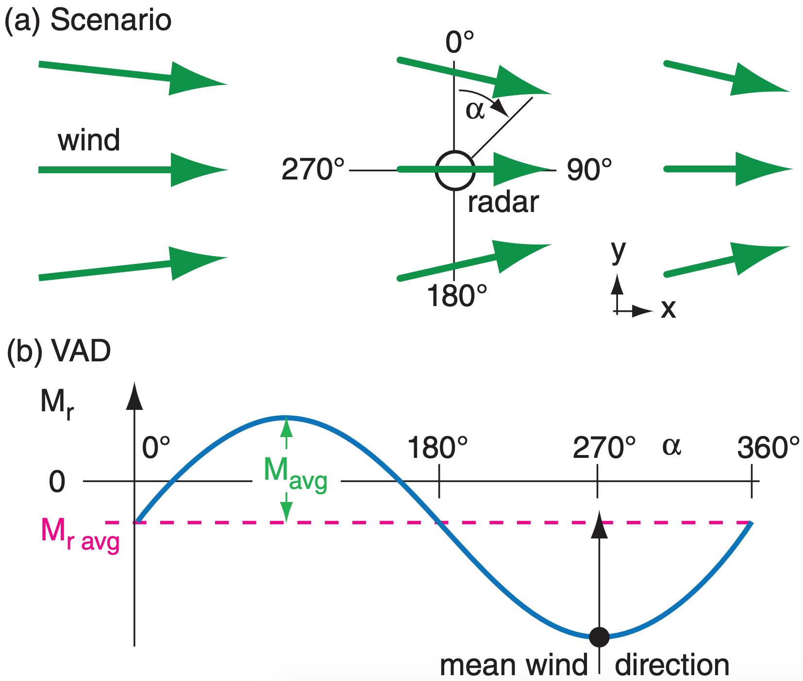
A plot of radial velocity Mr (at a fixed elevation angle and range) vs. azimuth angle α is called a velocity-azimuth display (VAD), which you can use to measure the mean horizontal wind speed and direction within that range circle. Fig. 8.36a illustrates a steady mean wind blowing from west to east through the Doppler radar sweep area. The resulting radial velocity component measured by the radar is a sine wave on the VAD (Fig. 8.36b).

Figure 8.36 (a) Scenario of mean winds relative to radar. (b) Velocity-azimuth display (VAD) of radial wind component. M_r is positive for wind AWAY from the radar.

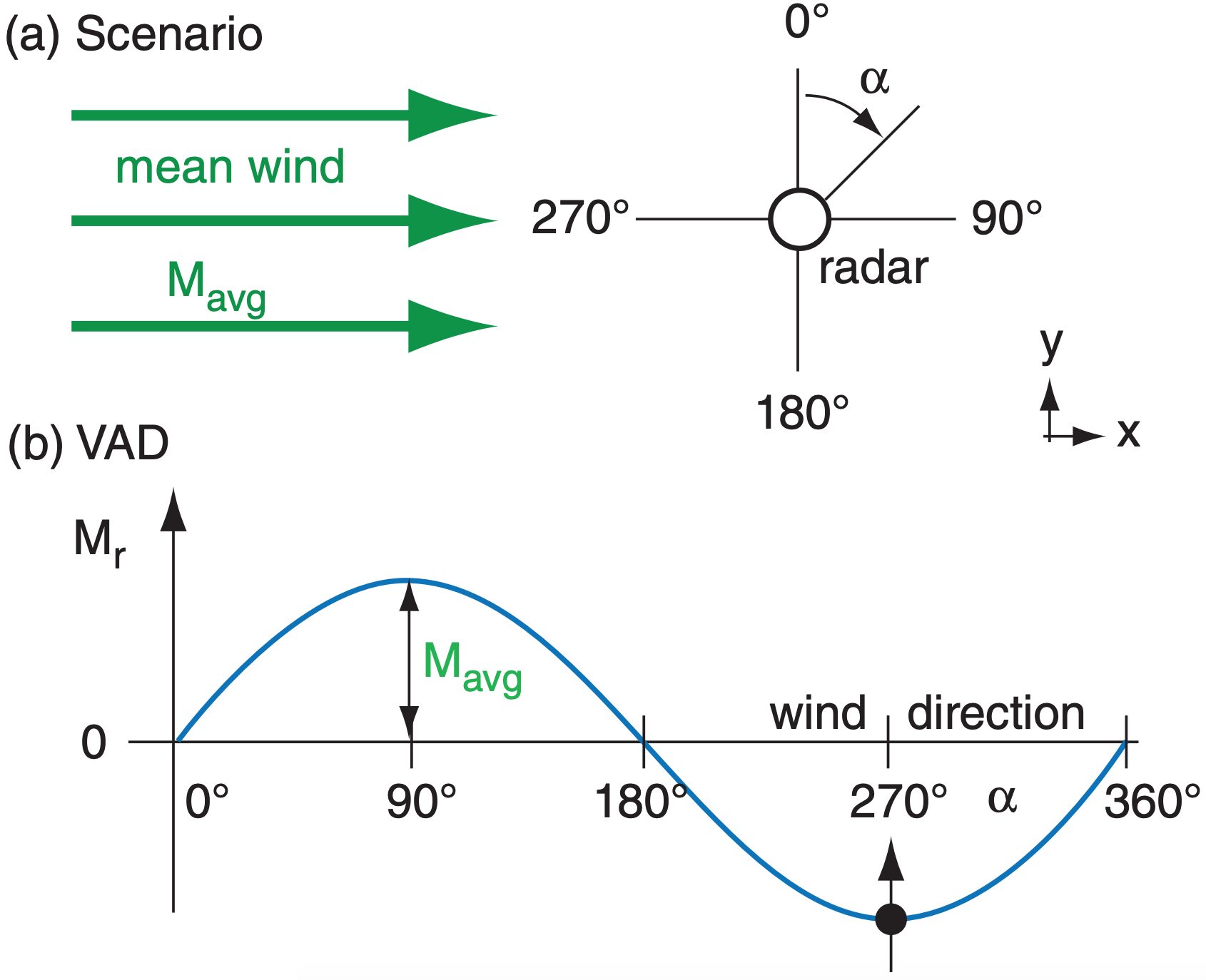
Mean horizontal wind speed M_avg is the amplitude of the sine wave relative to the average radial velocity M_{r avg} (=0 for this case), and the meteorological wind direction is the azimuth at which the VAD curve is most negative (Fig. 8.36b). Repeating this for different heights gives the winds at different altitudes, which you can plot as a wind-profile sounding or as a hodograph (explained in the Thunderstorm chapters). The measurements at different heights are made using different elevation angles and ranges (eq. 8.22).

You can also estimate mean vertical velocity using 2-D horizontal divergence determined from the VAD. Picture the scenario of Fig. 8.37a, where there is convergence (i.e., negative divergence) superimposed on the mean wind. Namely, west winds exist everywhere, but the departing winds east of the radar are slower than the approaching winds from the west. Also, the winds have a convergent north-south component. When plotted on a VAD, the result is a sine wave that is displaced in the vertical (Fig. 8.37b). Averaging the slower AWAY radial winds with the faster TOWARD radial winds gives a negative average radial velocity M_{r avg}, as shown by the dashed line in Fig. 8.37b. M_{r avg} is a measure of the divergence/convergence, while M_avg still measures mean wind speed.

Figure 8.37 (a) Scenario of mean winds AND 2-D horizontal convergence. (b) Velocity-azimuth display (VAD) of radial wind component.

Due to mass continuity (discussed in the Atmospheric Forces & Winds chapter), an accumulation of air horizontally into a volume requires upward motion of air out of the volume to conserve mass (i.e., mass flow in = mass flow out). Thus:

\(\ \begin{align} \Delta w=\frac{-2 \cdot M_{r a v g}}{R} \cdot \Delta z\tag{8.37}\end{align}\)

where ∆w is change in vertical velocity across a layer of thickness ∆z, and R is range from the radar at which the radial velocity M_r is measured.

Upward vertical velocities (associated with horizontal convergence and negative M_{r avg}) enhance cloud and storm development, while downward vertical velocities (subsidence, associated with horizontal divergence and positive M_{r avg}) suppress clouds and provide fair weather. Knowing that w = 0 at the ground, you can solve eq. (8.37) for w at height ∆z above ground. Then, starting with that vertical velocity, you can repeat the calculation using average radial velocities at a higher elevation angle to find w at this higher altitude. Repeating this gives the vertical velocity profile.

A single Doppler radar cannot measure the full horizontal wind field, because it can “see” only the radial component of velocity. However, if the scan regions of two nearby Doppler radars overlap, then in theory the horizontal wind field can be calculated from this dual-Doppler information, and the full 3-D winds can be inferred using mass continuity.

Sample Application

From a 1 km thick layer of air near the ground, the average radial velocity is –2 m s^–1 at range 100 km from the radar. What is the vertical motion at the layer top?

Find the Answer

Given: R = 100 km , ∆z = 1 km , M_{r avg} = –2 m s^–1.

Find: w = ? m s^–1 at z = 1 km.

Assume: w_bot = 0 at the ground (at z = 0).

Use eq. (8.37): ∆w = –2·(–2 m s^–1) · (1 km) / (100 km)

∆w = +0.04 m s^–1.

But ∆w = w_top – w_bot . Thus: w_top = +0.04 m s^–1

Check: Units OK. Physics OK.

Exposition: This weak upward motion covers a broad 100 km radius circle, and would enhance storms.

8.3.3.4. Identification of Storm Characteristics

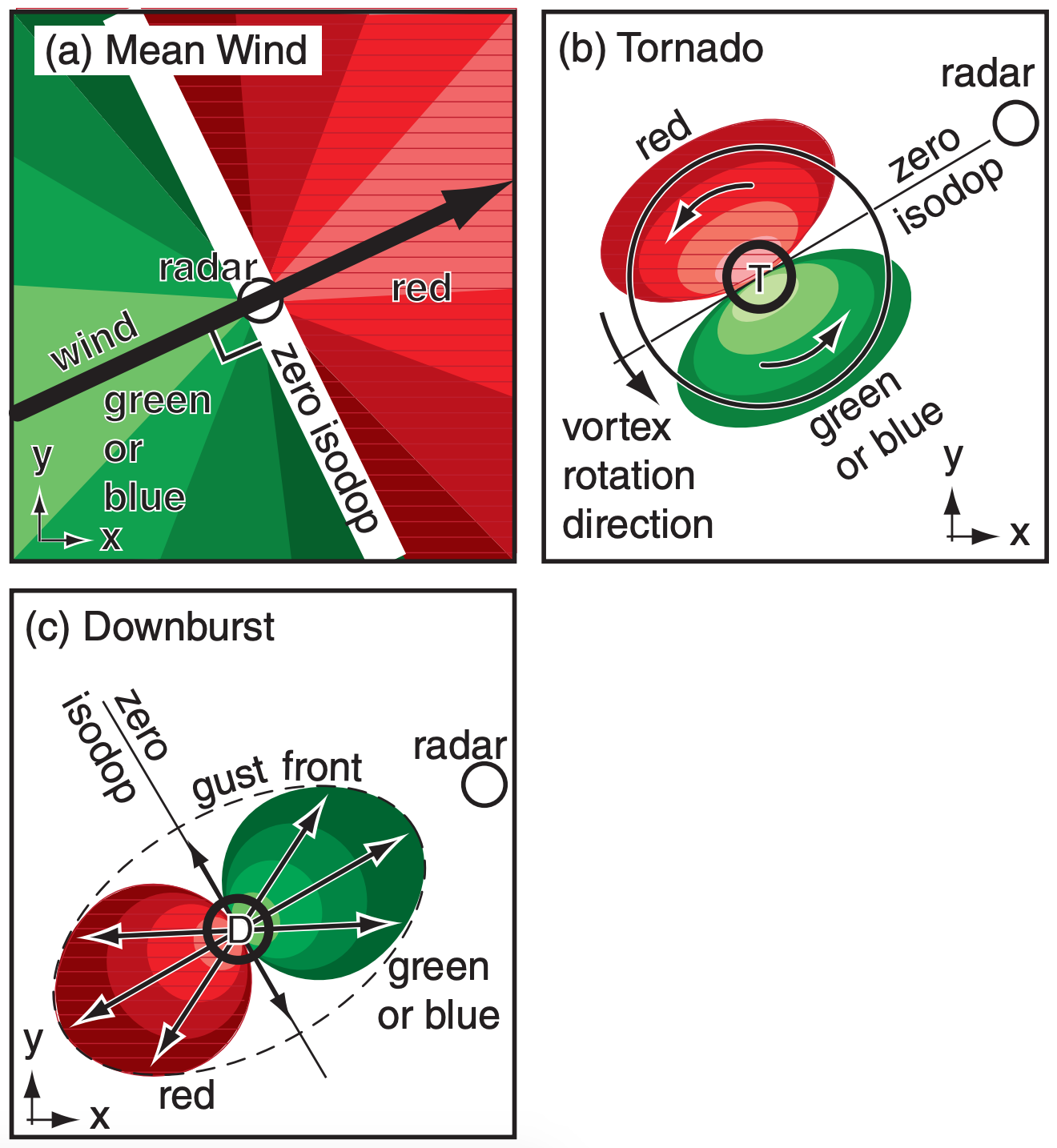
While the VAD approach averages the winds within the whole scan circle, you can also use the smaller scale patterns of winds to identify storm characteristics. For example, you can use Doppler information to help detect and give advanced warning for tornadoes and mesocyclones (see the Thunderstorm chapters). A single Doppler radar cannot see the whole rotation inside the thunderstorm — just the portions of the vortex with components moving toward or away from the radar. But you can use this limited information to define a tornado vortex signature (TVS, Fig. 8.38b) with the brightest red and green pixels next to each other, and with the zero isodop line passing through the tornado center and following a radial line from the radar.

Figure 8.38 PPI or CAPPI radar image interpretation. The white circle indicates the radar location. Red shaded regions indicate wind components AWAY from the radar. Green (or blue on some displays) indicate a wind components TOWARD the radar. Darker shadings represent slower radial wind components. Actual wind directions are shown by the black arrows. (a) Uniform mean wind in the domain. (b) Tornado T vortex, surrounded by weaker mesocyclone vortex (large circle). (c) Downburst D and gust front (dashed line) at the leading edge of outflow air.

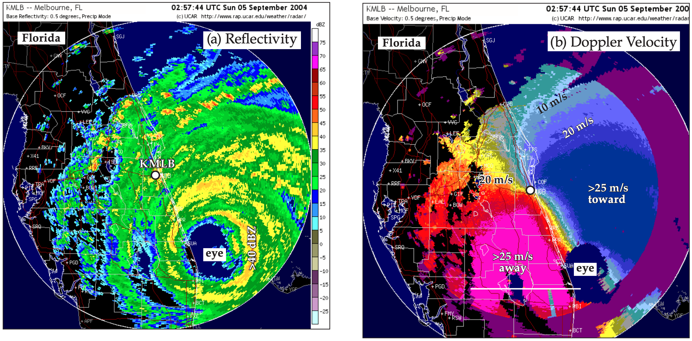
Hurricanes also exhibit these rotational characteristics, as shown in Fig. 8.39. Winds are rotating counterclockwise around the eye of this Northern Hemisphere hurricane. The zero isodop passes through the radar location in the center of this image, and also passes through the center of the eye of the hurricane. See the Tropical Cyclone chapter for details.

Cold-air downbursts from thunderstorms hit the ground and diverge (spread out) as damaging horizontal straight-line winds (Fig. 8.38c). The leading edge of the outflow is the gust front. Doppler radar sees this as neighboring regions of opposite moving radial winds, similar to the TVS but with the zero isodop perpendicular to the radial from the radar, and with the green region always closer to the radar than the red region.

Figure 8.39 Radar images of Hurricane Francis at 0300 UTC on 5 September 2004 as the eye is approaching the coast of Florida, USA. Hurricane intensity at this time was category 2 on the Saffir-Simpson scale, although it had been category 4 before reaching the coast. The Melbourne, FL, radar KMLB is in the center of the radar image, as indicated with the white dot. (a) PPI image of reflectivity (dBZ). (b) Doppler radial velocities. [Adapted from US National Weather Service data as displayed by the Research Applications Program division of the US National Center for Atmospheric Research.]

Sample Application

A downburst and outflow are centered directly over a Doppler radar. Sketch the Doppler display.

Find the Answer

Given: Air diverging in all directions from radar

Sketch: Doppler radar display appearance

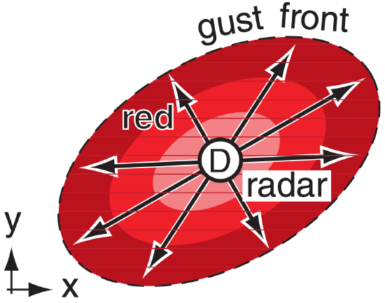At every azimuth from the radar, air is moving AWAY. Thus red would be all around the radar, out to the gust front. The fastest outflow (sketched as the lightest red) is likely to be closest to the radar.

Check: Sketch consistent with display definitions.

Exposition: Meteorologists at the radar might worry about their own safety, and about radome damage. The radome is the spherical enclosure that surrounds the radar antenna, to protect the radar from the weather. Also, a wet radome causes extra attenuation, making it difficult to see distant precipitation echoes.

8.3.3.5. Spectrum Width

Another product from Doppler radars is the spectrum width. This is the variance of the Doppler velocities within the sample volume, and is a measure of the intensity of atmospheric turbulence inside storms. Also, the Doppler signal can be used with reflectivity to help eliminate ground clutter. For high elevation angles and longer pulse lengths, the spectrum width is also large in bright bands, because the different fall velocities of rain and snow project onto different radial velocities. Strong wind shear within sample volumes can also increase the spectrum width.

8.3.3.6. Difficulties

Besides the maximum unambiguous velocity problem, other difficulties with Doppler-estimated winds are: (1) ground clutter including vehicles moving along highways or ocean waves approaching shore; (2) lack of information in parts of the atmosphere where there are no scatterers (i.e., no rain drops or bugs) in the air; and (3) scatterers that move at a different speed than the air, such as falling raindrops or migrating birds.

Sample Application

Explain the “S” shape of the portion of the zero isodop line that is close to the radar in Fig. 8.39b.

Find the Answer

Given: Doppler velocities in Fig. 8.39b.

Find: Explanation for “S” curve of zero isodop.

For a PPI display, the radar is observing the air along the surface of an inverted scan cone (Fig. 8.24a). Hence, targets at closer range to the radar correspond to targets at lower altitude. Curvature in the zero isodop indicates vertical shear of the horizontal winds (called wind shear for short).

Close to the radar the zero isodop is aligned northwest to southeast. The wind direction at low altitude is perpendicular to this direction; namely, from the northeast at low altitude.

Slightly farther from the radar (but still on the radar side of the eye), the zero isodop is south-southeast to the south of the radar, and is north-northwest on the north side. The winds at this range are perpendicular to a straight line drawn from the radar to the zero isodop; namely, the wind is from the east-northeast at mid altitudes.

Exposition: As you will see in the Winds & Hurricane chapters, boundary-layer winds feel the effect of drag against the ground, and have a direction that spirals in toward the eye. Above the boundary layer, in the middle of the troposphere, winds circle the eye.

8.3.4. Polarimetric Radar

Because Z-R relationships are inaccurate and do not give consistent results, other methods are used to improve estimates of precipitation type and rate. One method is to transmit microwave pulses with different polarizations, and then compare their received echo intensities. Radars with this capability are called polarimetric, dual-polarization, or polarization-diversity radars.

Recall that electromagnetic radiation consists of perpendicular waves in the electric and magnetic fields. Polarization is defined by the direction of the electric field. Radars can be designed to switch between two or three polarizations: horizontal, vertical, and circular (see Fig. 8.40). Air-traffic control radars use circular polarization, because it partially filters out the rain, allowing a clearer view of aircraft. Most weather radars use horizontal and vertical linear polarizations.

Figure 8.40 Polarization of microwaves, where E = electric field, M = magnetic field, and c = wave propagation at speed of light. (a) Vertical; (b) Horizontal; and (c) Circular polarization.

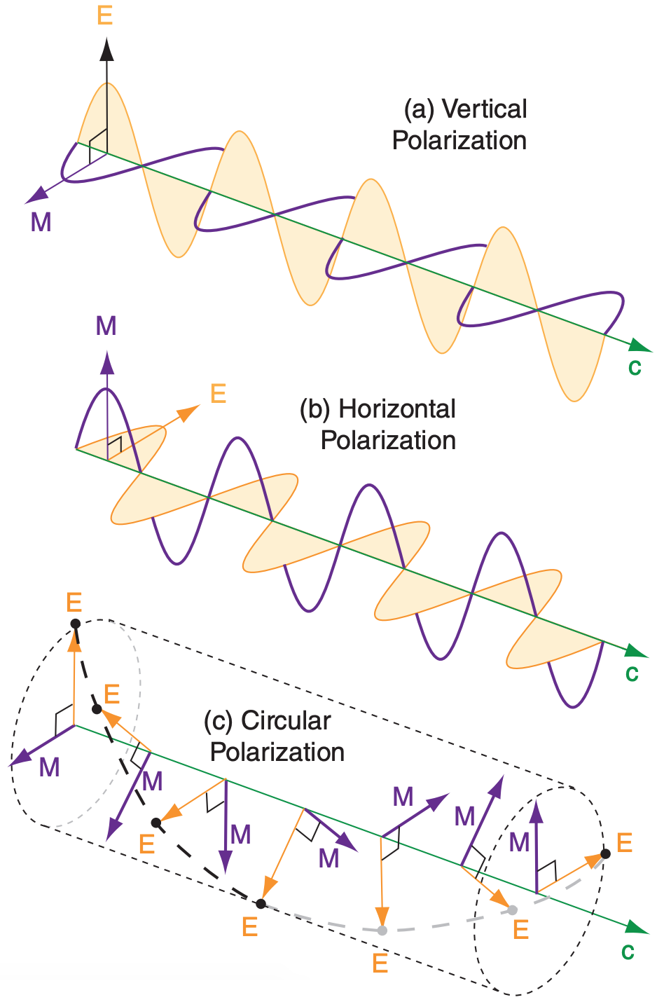
Horizontally polarized pulses get information about the horizontal dimension of the precipitation particles (because the energy scattered depends mostly on the particle horizontal size). Similarly, vertically polarized pulses get information about the vertical dimension. By alternating between horizontal and vertical polarization with each successive transmitted pulse, algorithms in the receiver can use echo differences to estimate the average shape of precipitation particles in the sample volume.

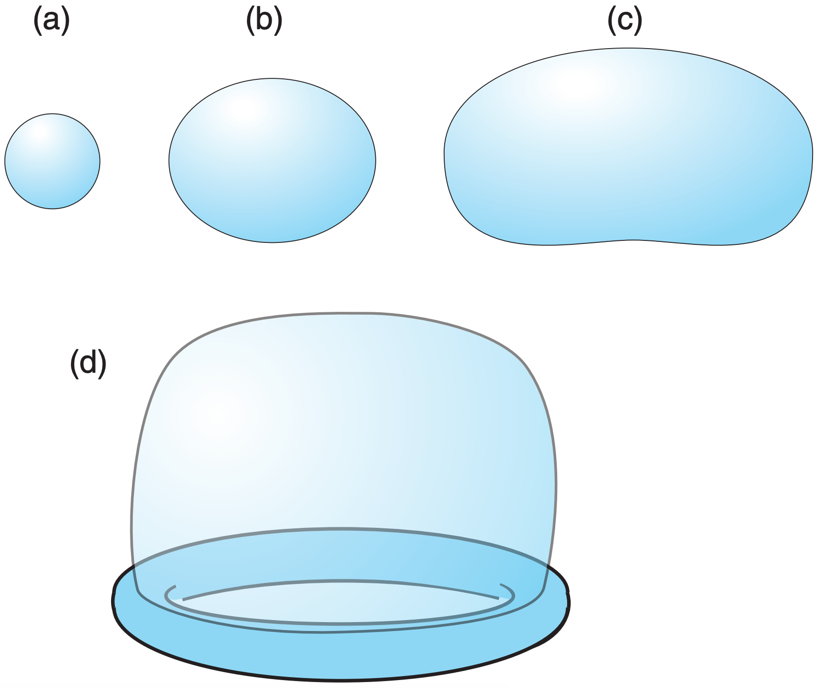
Only the smallest cloud droplets are spherical (Fig. 8.41a, equal width and height). These would give returns of equal magnitude for both horizontal and vertical polarizations. However, larger rain drops become more oblate (Fig. 8.41b, flattened on the bottom and top) due to air drag when they fall. The largest drops are shaped like a hamburger bun (Fig. 8.41c). This gives greater reflectivity factor Z_H from the horizontally polarized pulses than from the vertically polarized ones Z_V. The amount of oblateness increases with the mass of water in the drop. There is some evidence that just before the largest drops break up due to air drag, they have a parachute or jelly-fish-like shape (Fig. 8.41d).

Figure 8.41 Enlargement of raindrop shapes vs. diameter D (approximate). (a) D < 1 mm; (b) 1 mm < D < 3 mm ; (c) 3 mm < D; (d) large (D ≈ 4 mm) jellyfish-like shape just before drop breaks up..

Some hydrometeor shapes change the polarization of the scattered pulse. For example, clockwise circular polarized transmitted pulses are scattered with counterclockwise circular polarization by any rain drops that are nearly spherical. Tumbling, partially melted, irregularly shaped ice crystals can respond to horizontally polarized pulses by returning a portion of the energy in vertical polarization. Different shapes of ice crystals have different reflectivity factors in the vertical and horizontal.

Four variables are often analyzed and displayed on special radar images to help diagnose hydrometeor structure and size. These are:

• Differential Reflectivity: Z_DR (unit: dB)

  \(\ \begin{align} Z_{D R}=10 \cdot \log \left(Z_{H H} / Z_{V V}\right)\tag{8.38}\end{align}\)

  where the first and second subscripts of reflectivity Z on the right hand side give the polarization (H = horizontal; V = vertical) of received and transmitted pulses, respectively.

  Typical values: –2 to +6 dB, where negative and positive values indicate vertical or horizontal orientation of the hydrometeor’s major axis.

  Useful with Z for improving rain-rate estimates and identifying radar attenuation regions.

• Linear Depolarization Ratio. LDR (unit: dB) \(\ \begin{align} L D R=10 \cdot \log \left(Z_{V H} / Z_{H H}\right)\tag{8.39}\end{align}\)

  Typical values: > –10 dB for ground clutter

  –15 dB for melting snowflakes

  –20 to –26 dB for melting hail

  < –30 dB for rain

  Useful for estimating micrometeor type or habit. Can also help remove ground clutter and identify the bright band.

• Specific Differential Phase: K_DP

  Typical values: –1 to +6 °/km, where positive values indicate oblate (horizontally dominant) hydrometeors. Tumbling hail appears symmetric on average, resulting in K_DP = 0.

  Improves accuracy of rain rate estimate and helps to isolate the portion of echo associated with rain in a rain/hail mixture.

• Co-polar Correlation Coefficient: ρ_HV (unit: dimensionless, in range –1 to +1 ) Measures the amount of similarity in variation of the time series of received signals from the horizontal vs. vertical polarizations. Typical values of |ρ_HV|:

  0.5 means very large hail

  0.7 to 0.9 means drizzle or light rain

  0.90 to 0.95 means hail or bright-band mix

  ≥ 0.95 means rain, snow, ice pellets, graupel

  0.95 to 1.0 means rain

  Useful for estimating radar-beam attenuation and the heterogeneity of micrometeors (mixtures of differently shaped ice crystals and rain drops) in the sampling volume.

Sample Application

Polarization radar measures reflectivity factors of Z_HH = 1000 dBZ , Z_VV = 398 dBZ , and Z_VH = 0.3 dBZ. (a) Find the differential reflectivity and the linear depolarization ratio. (b) Discuss characteristics of the hydrometeors. (c) What values of specific differential phase and co-polar correlation coefficient would you expect? Why?

Find the Answer

Given: Z_HH = 1000 dBZ, Z_VV = 398 dBZ , and Z_VH = 0.3 dBZ

Find: Z_DR = ? dB, LDR = ? dB

(a) Use eq. (8.38): Z_DR = 10·log(1000 dBZ/398 dBZ) = +4.0 dB

Use eq. (8.39): LDR = 10·log(0.3 dBZ/1000 dBZ) = –35.2 dB

(b) Discussion: The positive value of Z_DR indicates a hydrometeor with greater horizontal than vertical dimension, such as large, oblate rain drops. The very small value of LDR supports the inference of rain, rather than snow or hail.

(c) I would expect K_DP = 2 to 4 °/km, because of large oblate rain drops.

I would also expect ρ_HV = 0.95 , because rain intensity is light to moderate, based on eq. (8.27):

dBZ = 10·log(Z_HH/Z₁)

= 10·log(1000dBZ/1dBZ)

= 30 dBZ, which is then used to find the intensity classification from Fig. 8.28.

Check: Units OK. Results reasonable for weather.

Exposition: See item (b) above.

In eq. (8.27) I used Z_HH because the horizontal drop dimension is the one that is best correlated with the mass of the drop, as illustrated in Fig. 8.41.

One suggestion for an improved estimate of rainfall rate RR with S-band polarimetric radar is:

\(\ \begin{align} R R=a_{0} \cdot K_{D P}^{a_{1}} \cdot Z_{D R}^{a_{2}}\tag{8.40}\end{align}\)

where a_o = 90.8 mm h^–1 (see Sample Application “check” for discussion of units), a₁ = 0.89, and a₂ = –1.69 . Such improved rainfall estimates are crucial for hydrometeorologists (experts who predict drought severity, river flow and flood potential).

Based on all the polarimetric information, fuzzy-logic algorithms are used at radar sites to classify the hydrometeors and to instantly display the result on computer screens for meteorologists. Hydrometeor Classification Algorithms (HCA) for WSR-88D radars use different algorithms for summer (warm mode) and winter (cold mode) precipitation.

• Warm Mode: big drops, hail, heavy rain, moderate rain, light rain, no echoes, birds/insects, anomalous propagation.
• Cold Mode: convective rain, stratiform rain, wet snow, dry snow, no echoes, birds/insects, anomalous propagation.

Combinations of polarimetric variables can also help identify graupel and estimate hail size, estimate attenuation of the radar signal, identify storms that might become electrically active (lots of lightning), identify regions that could cause hazardous ice accumulation on aircraft, detect tornado debris clouds, and correct for the bright band.

Sample Application

Polarization radar measures a differential reflectivity of 5 dB and specific differential phase of 4°/km. Estimate the rainfall rate.

Find the Answer

Given: Z_DR = 5 dB , K_DP = 4°/km.

Find: RR = ? mm h^–1

Use eq. (8.40):

RR = (90.8 mm h^–1) · (4°/km)^0.89 · (5 dB)^–1.69

= (90.8 mm h^–1)· 3.43 · 0.066 = 20 mm h^–1

Check: Units don’t match. The reason is that the units of a_o are not really [mm/h], but are [(mm h^–1) · (°/km)^–0.89 · (dB)^+1.69 ]. These weird units resulted from an empirical fit of the equation to data, rather than from first principles of physics.

Exposition: This corresponds to heavy rain (Fig. 8.28), so hydrometeorologists would try to forecast the number of hours that this rain would continue to estimate the storm-total accumulation (= rainfall rate times hours of rain). If excessive, they might issue a flood warning.

8.3.5. Phased-Array Radars & Wind Profilers

Phased-array radars steer the radar beam not by rotating the antenna dish, but by using multiple transmitter heads that can transmit at slightly different times. Picture the radar housing viewed from above as the rectangle in Fig. 8.42a. On one side of the housing are an array of microwave transmitters (black dots in the Fig.). When any transmitter fires, it emits a wave front shown by the thin semicircle. If all transmitters fire at the same time, then the superposition of all the waves yield the most energy in an effective wave front (thick grey line) that propagates perpendicularly away from the transmitter housing, as shown by the grey arrow. For the example in Fig. 8.42a, the effective wave front moves east.

But these transmitters can also be made to fire sequentially (i.e., slightly out of phase with each other) instead of simultaneously (Fig. 8.42b). Suppose transmitter 1 fires first, and then a couple nanoseconds later transmitter 2 fires, and so on. A short time after transmitter 5 fires, its wave front (thin semicircle) has had time to propagate only a short distance, however the wave fronts from the other transmitters have been propagating for a longer time, and are further away from the housing. The superposition of the individual wave fronts now yields an effective wave front (thick grey line) that is propagating toward the southeast.

Figure 8.42 Phased array radar concept. Black dots represent transmitters.

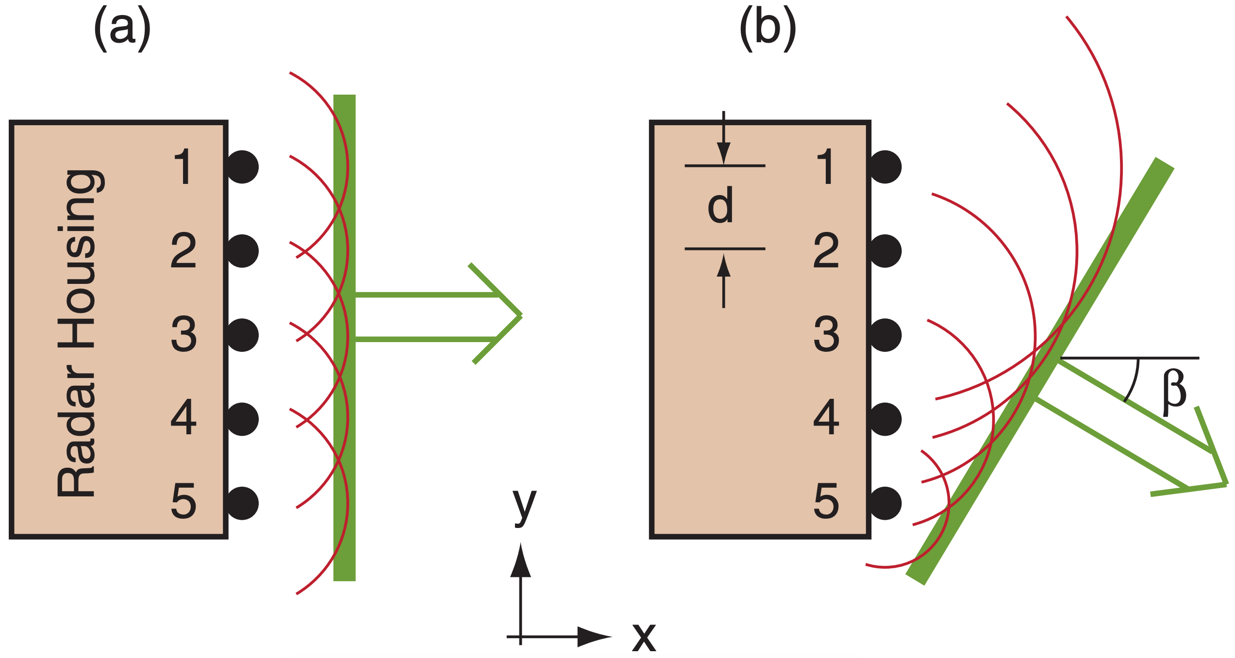
Let ∆t be the time delay between firing of subsequent transmitters. For transmitter elements spaced a distance d from each other, the time delay needed to give an effective propagation angle β (see Fig. 8.42b) is:

\(\ \begin{align} \Delta t=(d / c) \cdot \sin (\beta)\tag{8.41}\end{align}\)

where c ≈ 3x10⁸ m s^–1 is the approximate speed of microwaves through air.

By changing ∆t, the beam (grey arrow) can be steered over a wide range of angles. Negative ∆t steers the beam toward the northeast, rather than southeast in this example. Also, by having a 2-D array of transmitting elements covering the whole side of the housing, the beam can also be steered upward by firing the bottom elements first.

Sample Application

What time delay is needed in phased array radar to steer the beam 30° away from the line normal (perpendicular) to the radar face, if the transmitter elements are 1 m apart?

Find the Answer

Given: β = 30°, d = 1 m , c = 3x10⁸ m s^–1

Find: ∆t = ? s

Use eq. (8.41): ∆t = [(1m)/(3x10⁸ m s^–1)]·sin(30°)

∆t = 1.67x10^–9 s = 1.67 ns.

Check: Units OK. Physics OK. Agrees with Fig. 8.42.

Exposition: The larger the angle β, the smaller the effective size of the transmitter face, and the less focused is the beam. This is a disadvantage of phasedarray radars used for meteorology: the sample volume changes not only with range but also with direction β. Therefore, the algorithms used to interpret meteorological characteristics (reflectivity, Doppler velocity, spectrum width, polarimetric data) must be modified to account for these variations.

Two advantages of this approach are: (1) fewer moving parts, therefore less likelihood of mechanical failure; and (2) the beam angle can be changed instantly — allowing faster scans. However, to see a full 360° azimuth around the radar site, phased-array transmitting elements must be designed into all 4 outside walls of the radar building. While the military have used phased array radars for decades to detect aircraft and missiles, these radars are just beginning to be used in civilian meteorology. The US National Weather Service hopes to replace their 1988-vintage WSR-88D radars with modern multi-function phased-array weather radars.

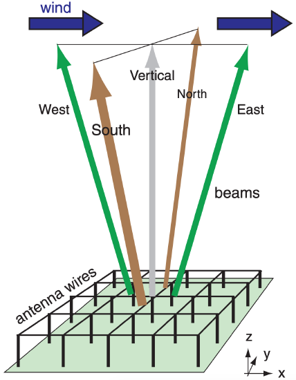
Another phased-array application to meteorology is the wind profiler. This observes horizontal wind speed and direction at many heights by measuring the Doppler shifts in the returned signals from a set of radio beams tilted slightly from vertical (Fig. 8.43).

Figure 8.43 Wind profiler concept.

Some wind profilers look like a forest of TV antennas sticking out of the ground, others like window blinds laying horizontally, others like a large trampoline, and others like a grid of perpendicular clothes lines on poles above the ground (Fig. 8.43). Each line is a radio transmitter antenna, and the effective beam can be steered away from vertical by phased (sequential) firing of these antenna wires.

Wind profilers work somewhat like radars — sending out pulses of radio waves and determining the height to the clear-air targets by the time delay between transmitted and received pulses. The targets are turbulent eddies of size equal to half the radio wavelength. These eddies cause refractivity fluctuations that scatter some of the radio-wave energy back to receivers on the ground; hence, bugs or raindrops are not needed as targets.

Wind profilers with 16 km altitude range use Very High Frequencies (VHF) of about ν = 50 MHz (λ = c/ν = 6 m). Other tropospheric wind profilers use an Ultra High Frequency (UHF) near 400 MHz (λ = 0.75 m = 75 cm). Smaller boundary-layer wind profilers for sampling the lower troposphere use an ultra high frequency near 1 GHz (λ = 30 cm).

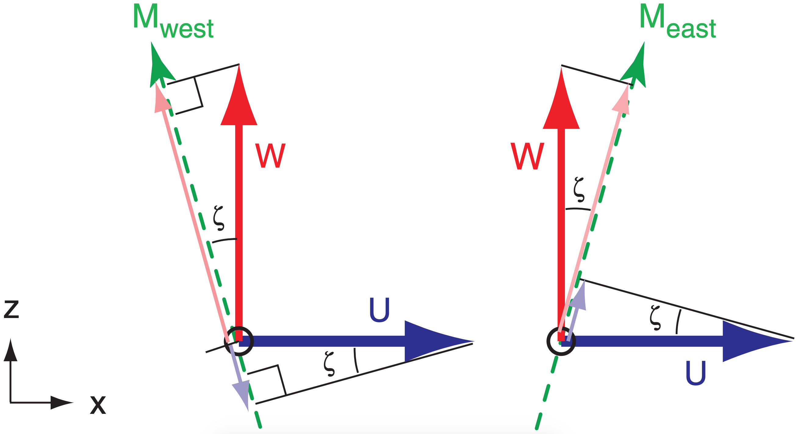
Normally, wind profilers are designed to transmit in only 3, 4 or 5 nearly-vertical, fixed beam directions (Fig. 8.43). The fixed zenith angle of the slightly tilted beams is on the order of ζ = 14° to 24°.

The radial velocities M_east and M_west measured in the east- and west-tilted beams, respectively, are affected by the U component of horizontal wind and by vertical velocity W. Positive W (upward motion; thick grey vector in Fig. 8.44) projects into positive (away from wind profiler) components of radial velocity for both beams (thin grey vectors). However, positive U (thick black vector) wind contributes positively to M_east, but negatively (toward the profiler) to M_west (thin black vectors).

Assume that both beams measure the same air parcel at nearly the same instant, and thus detect the same average U and W. Design the profiler so that all tilted beams have the same zenith angle. Use the measured radial velocities from a pair of oppositely tilted beams. By adding and subtracting these two measured velocities ( M_east , M_west ), you can solve for the desired wind components (U, W):

\(\ \begin{align} U=\frac{M_{e a s t}-M_{w e s t}}{2 \cdot \sin \zeta}\tag{8.42a}\end{align}\)

\(\ \begin{align} W=\frac{M_{e a s t}+M_{w e s t}}{2 \cdot \cos \zeta}\tag{8.42b}\end{align}\)

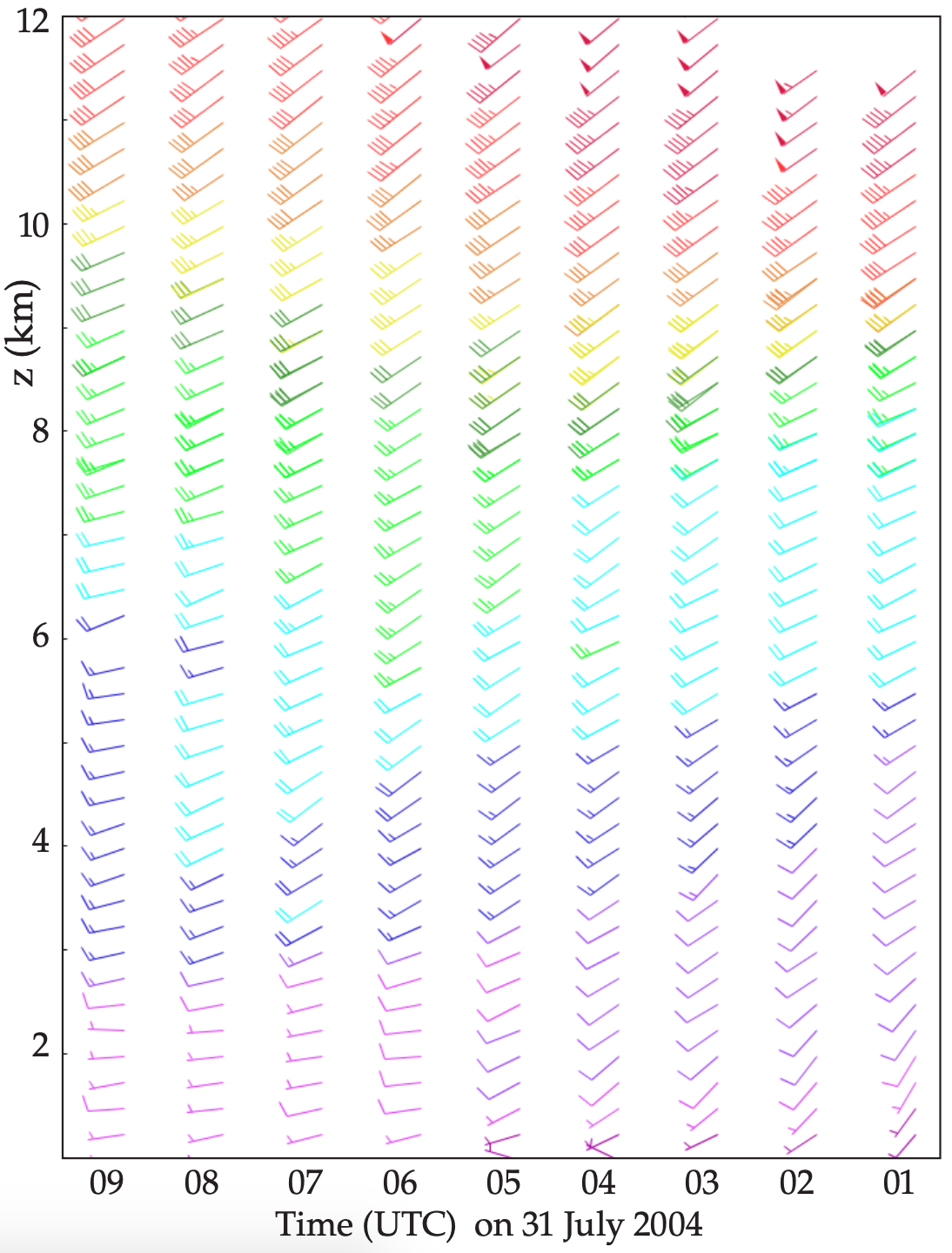
Use similar equations with radial velocities from the north- and south-tilted beams to estimate V and W. Fig. 8.45 shows sample wind-profiler output.

Figure 8.44 Projections of horizontal wind U and vertical velocity W to the radial wind directions M_west and M_east along wind-profiler west- and east-tilted beams. M_west and M_east are positive when pointed upward.

Figure 8.45 Wind profiler observations for Wolcott, IN. Arrow shows horizontal wind direction. Each short wind barb = 5 m/s, long = 10 m/s, & pennant = 50 m/s. (E.g., wind at z = 10 km, t = 02 UTC is 45 m/s from southwest.) Courtesy of US National Oceanic and Atmospheric Admin. (NOAA) Profiler Network (NPN).

Sample Application

A wind profiler with 20° beam tilt uses the Doppler shift to measure radial velocities of 3.326 m s^–1 and –3.514 m s^–1 in the east- and west-tilted beams, respectively, at height 4 km above ground. Find the vertical and horizontal wind components at that height.

Find the Answer

Given: M_east= 3.326 m s^–1, M_west= –3.514 m s^–1, ζ = 20°

Find: U = ? m s^–1 and W = ? m s^–1.

Use eq. (8.42a):

U = [(3.326 m s^–1) – (–3.514 m s^–1)]/[2·sin(20°)]=10 m s^–1

Use eq. (8.42b):

W=[(3.326 m s^–1)+(–3.514 m s^–1)]/[2·cos(20°)]=–0.1 m s^–1

Check: Units OK. Physics OK.

Exposition: The positive U component indicates a west wind (i.e., wind FROM the west) at z = 4 km. Negative W indicates subsidence (downward moving air). These are typical of fair-weather conditions under a strong high-pressure system. Typical wind profilers make many measurements each minute, and then average their results over 5 minutes to 1 hour.