
17.3: Thermally Driven Circulations
- Page ID
- 9640

\( \newcommand{\vecs}[1]{\overset { \scriptstyle \rightharpoonup} {\mathbf{#1}} } \)
\( \newcommand{\vecd}[1]{\overset{-\!-\!\rightharpoonup}{\vphantom{a}\smash {#1}}} \)
\( \newcommand{\dsum}{\displaystyle\sum\limits} \)
\( \newcommand{\dint}{\displaystyle\int\limits} \)
\( \newcommand{\dlim}{\displaystyle\lim\limits} \)
\( \newcommand{\id}{\mathrm{id}}\) \( \newcommand{\Span}{\mathrm{span}}\)
( \newcommand{\kernel}{\mathrm{null}\,}\) \( \newcommand{\range}{\mathrm{range}\,}\)
\( \newcommand{\RealPart}{\mathrm{Re}}\) \( \newcommand{\ImaginaryPart}{\mathrm{Im}}\)
\( \newcommand{\Argument}{\mathrm{Arg}}\) \( \newcommand{\norm}[1]{\| #1 \|}\)
\( \newcommand{\inner}[2]{\langle #1, #2 \rangle}\)
\( \newcommand{\Span}{\mathrm{span}}\)
\( \newcommand{\id}{\mathrm{id}}\)
\( \newcommand{\Span}{\mathrm{span}}\)
\( \newcommand{\kernel}{\mathrm{null}\,}\)
\( \newcommand{\range}{\mathrm{range}\,}\)
\( \newcommand{\RealPart}{\mathrm{Re}}\)
\( \newcommand{\ImaginaryPart}{\mathrm{Im}}\)
\( \newcommand{\Argument}{\mathrm{Arg}}\)
\( \newcommand{\norm}[1]{\| #1 \|}\)
\( \newcommand{\inner}[2]{\langle #1, #2 \rangle}\)
\( \newcommand{\Span}{\mathrm{span}}\) \( \newcommand{\AA}{\unicode[.8,0]{x212B}}\)
\( \newcommand{\vectorA}[1]{\vec{#1}} % arrow\)
\( \newcommand{\vectorAt}[1]{\vec{\text{#1}}} % arrow\)
\( \newcommand{\vectorB}[1]{\overset { \scriptstyle \rightharpoonup} {\mathbf{#1}} } \)
\( \newcommand{\vectorC}[1]{\textbf{#1}} \)
\( \newcommand{\vectorD}[1]{\overrightarrow{#1}} \)
\( \newcommand{\vectorDt}[1]{\overrightarrow{\text{#1}}} \)
\( \newcommand{\vectE}[1]{\overset{-\!-\!\rightharpoonup}{\vphantom{a}\smash{\mathbf {#1}}}} \)
\( \newcommand{\vecs}[1]{\overset { \scriptstyle \rightharpoonup} {\mathbf{#1}} } \)
\(\newcommand{\longvect}{\overrightarrow}\)
\( \newcommand{\vecd}[1]{\overset{-\!-\!\rightharpoonup}{\vphantom{a}\smash {#1}}} \)
\(\newcommand{\avec}{\mathbf a}\) \(\newcommand{\bvec}{\mathbf b}\) \(\newcommand{\cvec}{\mathbf c}\) \(\newcommand{\dvec}{\mathbf d}\) \(\newcommand{\dtil}{\widetilde{\mathbf d}}\) \(\newcommand{\evec}{\mathbf e}\) \(\newcommand{\fvec}{\mathbf f}\) \(\newcommand{\nvec}{\mathbf n}\) \(\newcommand{\pvec}{\mathbf p}\) \(\newcommand{\qvec}{\mathbf q}\) \(\newcommand{\svec}{\mathbf s}\) \(\newcommand{\tvec}{\mathbf t}\) \(\newcommand{\uvec}{\mathbf u}\) \(\newcommand{\vvec}{\mathbf v}\) \(\newcommand{\wvec}{\mathbf w}\) \(\newcommand{\xvec}{\mathbf x}\) \(\newcommand{\yvec}{\mathbf y}\) \(\newcommand{\zvec}{\mathbf z}\) \(\newcommand{\rvec}{\mathbf r}\) \(\newcommand{\mvec}{\mathbf m}\) \(\newcommand{\zerovec}{\mathbf 0}\) \(\newcommand{\onevec}{\mathbf 1}\) \(\newcommand{\real}{\mathbb R}\) \(\newcommand{\twovec}[2]{\left[\begin{array}{r}#1 \\ #2 \end{array}\right]}\) \(\newcommand{\ctwovec}[2]{\left[\begin{array}{c}#1 \\ #2 \end{array}\right]}\) \(\newcommand{\threevec}[3]{\left[\begin{array}{r}#1 \\ #2 \\ #3 \end{array}\right]}\) \(\newcommand{\cthreevec}[3]{\left[\begin{array}{c}#1 \\ #2 \\ #3 \end{array}\right]}\) \(\newcommand{\fourvec}[4]{\left[\begin{array}{r}#1 \\ #2 \\ #3 \\ #4 \end{array}\right]}\) \(\newcommand{\cfourvec}[4]{\left[\begin{array}{c}#1 \\ #2 \\ #3 \\ #4 \end{array}\right]}\) \(\newcommand{\fivevec}[5]{\left[\begin{array}{r}#1 \\ #2 \\ #3 \\ #4 \\ #5 \\ \end{array}\right]}\) \(\newcommand{\cfivevec}[5]{\left[\begin{array}{c}#1 \\ #2 \\ #3 \\ #4 \\ #5 \\ \end{array}\right]}\) \(\newcommand{\mattwo}[4]{\left[\begin{array}{rr}#1 \amp #2 \\ #3 \amp #4 \\ \end{array}\right]}\) \(\newcommand{\laspan}[1]{\text{Span}\{#1\}}\) \(\newcommand{\bcal}{\cal B}\) \(\newcommand{\ccal}{\cal C}\) \(\newcommand{\scal}{\cal S}\) \(\newcommand{\wcal}{\cal W}\) \(\newcommand{\ecal}{\cal E}\) \(\newcommand{\coords}[2]{\left\{#1\right\}_{#2}}\) \(\newcommand{\gray}[1]{\color{gray}{#1}}\) \(\newcommand{\lgray}[1]{\color{lightgray}{#1}}\) \(\newcommand{\rank}{\operatorname{rank}}\) \(\newcommand{\row}{\text{Row}}\) \(\newcommand{\col}{\text{Col}}\) \(\renewcommand{\row}{\text{Row}}\) \(\newcommand{\nul}{\text{Nul}}\) \(\newcommand{\var}{\text{Var}}\) \(\newcommand{\corr}{\text{corr}}\) \(\newcommand{\len}[1]{\left|#1\right|}\) \(\newcommand{\bbar}{\overline{\bvec}}\) \(\newcommand{\bhat}{\widehat{\bvec}}\) \(\newcommand{\bperp}{\bvec^\perp}\) \(\newcommand{\xhat}{\widehat{\xvec}}\) \(\newcommand{\vhat}{\widehat{\vvec}}\) \(\newcommand{\uhat}{\widehat{\uvec}}\) \(\newcommand{\what}{\widehat{\wvec}}\) \(\newcommand{\Sighat}{\widehat{\Sigma}}\) \(\newcommand{\lt}{<}\) \(\newcommand{\gt}{>}\) \(\newcommand{\amp}{&}\) \(\definecolor{fillinmathshade}{gray}{0.9}\)17.3.1. Thermals
Thermals are warm updrafts of air, rising due to their buoyancy. Thermal diameters are nearly equal to their depth, zi (Fig. 17.6).
A rising thermal feels drag against the surrounding environmental air (not against the ground). This drag is proportional to the square of the thermal updraft velocity relative to its environment. Neglecting advection and pressure deviations, the equation of vertical velocity W from the Atmospheric Forces & Winds chapter reduces to:
\(\ \begin{align} \dfrac{\Delta W}{\Delta t}=\dfrac{\theta_{v p}-\theta_{v e}}{\bar{T}_{v e}} \cdot|g|-C_{w} \dfrac{W^{2}}{z_{i}}\tag{17.3}\end{align}\)
\(\ tendency \quad buoyancy \quad turb.drug \)
where zi is the mixed-layer (boundary-layer) depth, Cw ≈ 5 is the vertical drag coefficient, θv is the virtual potential temperature, subscripts p and e indicate the air parcel (the thermal) and the environment, \(\overline{T_{v e}}\) is average absolute virtual temperature of the environment, and |g|= 9.8 m·s–2 is the magnitude of gravitational acceleration.
At steady state, the acceleration is near zero (∆W/∆t ≈ 0). Eq. (17.3) can be solved for the updraft speed of buoyant thermals (i.e., of warm air parcels):
\(\ \begin{align} W=\sqrt{\dfrac{|g| \cdot z_{i}}{C_{w}} \dfrac{\left(\theta_{v p}-\theta_{v e}\right)}{\bar{T}_{v e}}}\tag{17.4}\end{align}\)
Thus, warmer thermals in deeper boundary layers have greater updraft speeds.
This equation also applies to deeper convection at the synoptic- and meso-scales, such as weak updrafts in thunderstorms that rise to the top of the troposphere. For that case, zi is the depth of the troposphere, and the temperature difference is that between the mid-cloud and the surrounding environment at the same height. For stronger updrafts and downdrafts in thunderstorms, the pressure deviation term of the equation of vertical motion must also be included (see the Thunderstorm chapters).
Sample Application
Find the steady-state updraft speed in the middle of (a) a thermal in a boundary layer that is 1 km thick; and (b) a thunderstorm in a 11 km thick troposphere. Virtual temperature excess is 2°C for the thermal & 5°C for the thunderstorm, and \(|g| / \overline{T_{v e}}=0.0333 \mathrm{m} \cdot \mathrm{s}^{-2} \cdot \mathrm{K}^{-1}\)
Find the Answer
Given: \(|g| / \overline{T_{v e}}=0.0333 \mathrm{m} \cdot \mathrm{s}^{-2} \cdot \mathrm{K}^{-1}\)
(a) zi = 1000 m, Tvp – Tve = 2°C
(b) zi = 11,000 m, Tvp – Tve = 5°C,
Find: W = ? m s–1
Use eq. (17.4): (a) For the thermal:
\(W=\sqrt{\dfrac{\left(0.0333 \mathrm{m} \cdot \mathrm{s}^{-2} \mathrm{K}^{-1}\right)(1000 \mathrm{m})(2 \mathrm{K})}{5}}=\underline{\bf{3.65ms^{-1}}}\)
(b) For the thunderstorm:
\(W=\sqrt{\dfrac{\left(0.0333 \mathrm{m} \cdot \mathrm{s}^{-2} \mathrm{K}^{-1}\right)(11000 \mathrm{m})(5 \mathrm{K})}{5}}=\underline{\mathbf{19.1 ms^{-1}}}\)
Check: Units OK. Physics OK.
Exposition: These speeds are rough estimates. Between the updrafts are larger-diameter, slower downdrafts, so that air mass is conserved across any arbitrary horizontal plane. Convection (regions of up- and downdrafts) cause bumpy airplane rides.
17.3.2. Cross-valley Circulations
(Circulations perpendicular to the valley axis.)
17.3.2.1. Anabatic Wind
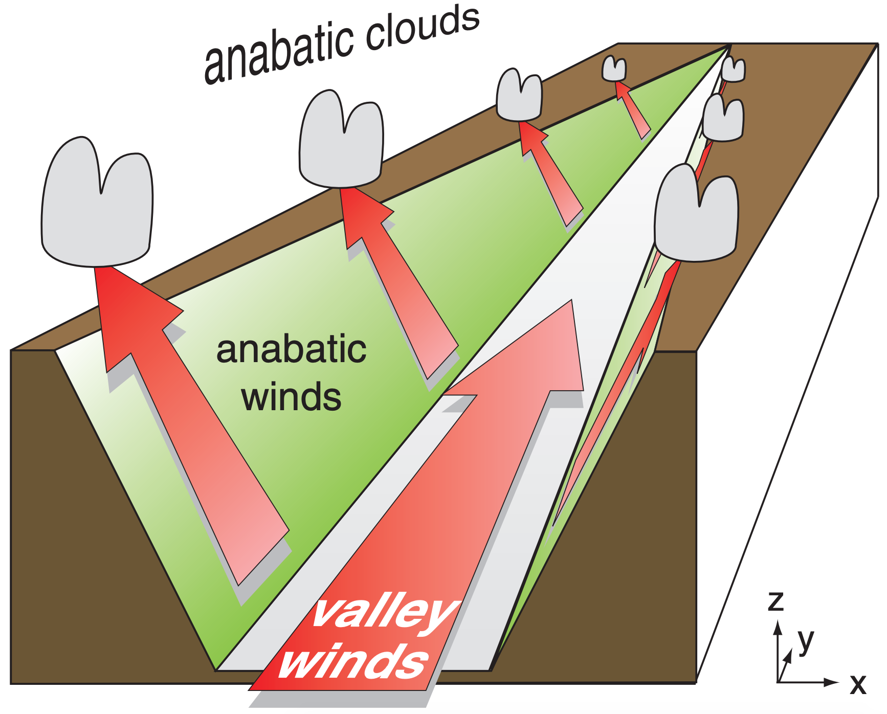
During daytime in synoptically calm conditions (high-pressure center) with mostly clear skies, the sunlight heats mountain slopes. The warm mountain surface heats the neighboring air, which then rises. However, instead of rising vertically like thermals, the rising air hugs the slope as it rises. This warm turbulent air rising upslope is called an anabatic wind (Fig. 17.7). Typical speeds are 3 to 5 m s–1, and depths are hundreds of meters. The anabatic wind is the rising portion of a cross-valley circulation.
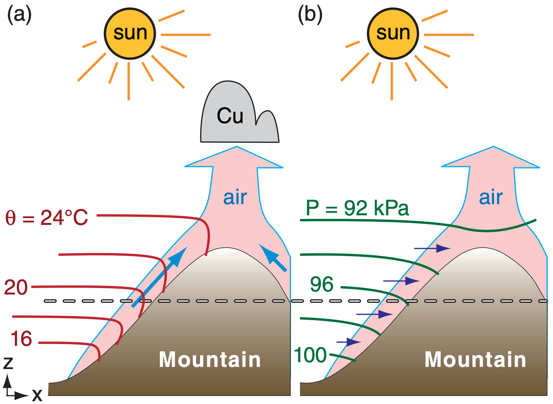
When the warm air reaches ridge top, it breaks away from the mountain and rises vertically, often joined by the updraft from the other side of the same mountain. Cumulus clouds called anabatic clouds can form just above ridge top in this updraft.
The dashed line in Fig. 17.7 is at a constant height above sea level. Following the line from left to right in Fig. 17.7a, potential temperatures of about 19°C are constant until reaching anabatic air near the mountain, where the potential temperature rises to about 21°C in this idealized illustration.
The temperature difference between the warmed air near the mountain and the cooler ambient air creates a small horizontal pressure gradient force (exaggerated in Fig. 17.7b) that holds the warm rising air against the mountain. To find this horizontal pressure-gradient force per unit mass m, use the hypsometric equation (see INFO box on next page):
\(\ \begin{align} \dfrac{F_{x P G}}{m}=-\dfrac{1}{\rho} \dfrac{\Delta P}{\Delta x}=|g| \dfrac{\Delta T}{T_{e}} \cdot \tan (\alpha)\tag{17.5}\end{align}\)
where ∆x is horizontal distance (positive in the uphill direction), |g|= 9.8 m·s–2 is gravitational acceleration magnitude, ∆T = Tp – Te is temperature difference between the air near and far from the slope, Tp is temperature of the warm near-mountain air, Te is temperature of the cooler environmental air, and α is the mountain slope angle. Use absolute temperature (kelvins) in the denominator of eq. (17.5).
The horizontal pressure difference across the anabatic flow is very small compared to the vertical pressure difference of air in hydrostatic balance. However, the horizontal pressure difference occurs across a short horizontal distance (tens of meters), yielding a modest pressure gradient that drives a measurable anabatic wind.
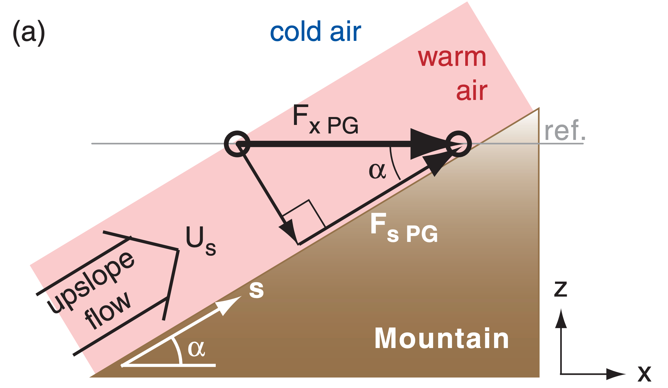
The portion of this pressure-gradient force in the along-slope direction (s) is Fs PG = Fx PG · cos(α), as can be seen from Fig. 17.8a. Combining this with the previous equation, and using the trigonometric identity tan(α) · cos(α) = sin(α), gives:
\(\ \begin{align} \dfrac{F_{s} P G}{m}=|g| \dfrac{\Delta T}{T_{e}} \cdot \sin (\alpha)\tag{17.6}\end{align}\)
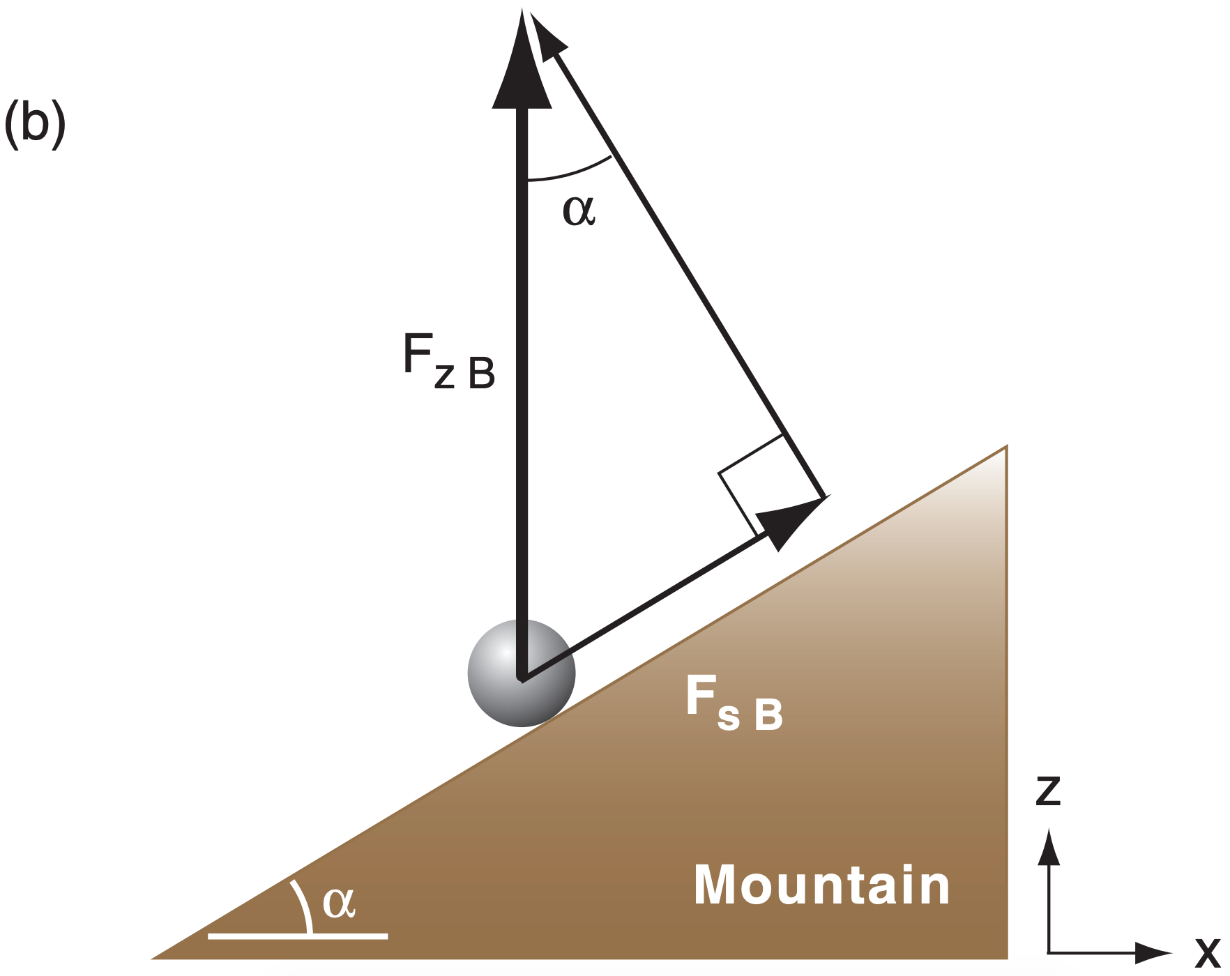
But recall from the vertical equation of motion that the vertical buoyancy force is FzB/m = |g|·(∆T/Te). Thus, eq. (17.6) can also be interpreted as the component of vertical buoyancy force in the up-slope direction (s), as can be seen from Fig. 17.8b.
Sample Application
Anabatic flow is 5°C warmer than the ambient environment of 15°C. Find the horizontal and alongslope pressure-gradient forces/mass, for a 30° slope.
Find the Answer
Given: Te = 15°C + 273 = 288 K, ∆T = 5 K, α = 30°
Find: (a) FxPG/m = ? m·s–2, (b) FsPG/m = ? m·s–2
|g|·∆T/Te = (9.8m·s–2)·(5K)/(288K) = 0.17 m·s–2
Use eq. (17.5): Fx PG/m = (0.17 m·s–2)·tan(30°) = 0.098 m·s–2
Use eq. (17.6): Fs PG/m = (0.17 m·s–2)·sin(30°) = 0.085 m·s–2
Check: Units OK, because m·s–2 = N kg–1.
Exposition: Glider and hang-glider pilots use the anabatic updrafts to soar along mountain slopes and mountain tops.
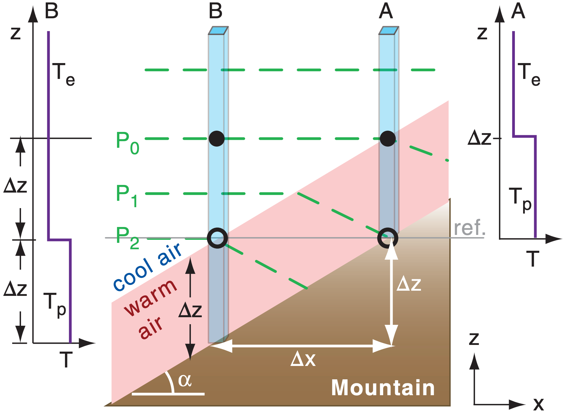
Derivation of Horizontal Pressure Gradient
Consider an idealized situation of isothermal environmental air of temperature Te and warmer near-mountain air (shaded grey) of temperature Tp with uniform vertical depth ∆z, as sketched in Fig. 17.b. Consider two air columns: A and B. If a reference height ref is set at the base of column A (thin grey line), then place column B such that the same ref height is at the top of the warm-air layer.
For both columns A and B, start at the same pressure (Po, at the solid black dots in Fig. 17.b). As you descend distance ∆z, the pressure P increase depends on air temperature T, as given by the hypsometric equation (from Chapter 1):
\(\ \begin{align} \ln (P)=\ln \left(P_{o}\right)+\dfrac{\Delta z}{a \cdot T}\tag{1}\end{align}\)
where a = ℜd/|g| = 29.3 m K–1. Thus, the ln(P) increases linearly with decreasing altitude (Fig. 17.c).
In column B, the temperature is uniformly cool between the solid black dot and the reference height, so pressure increases rapidly as you descend (Fig. 17.c). However, in column A, the temperature is uniformly warmer, so the pressure doesn’t increase as fast.
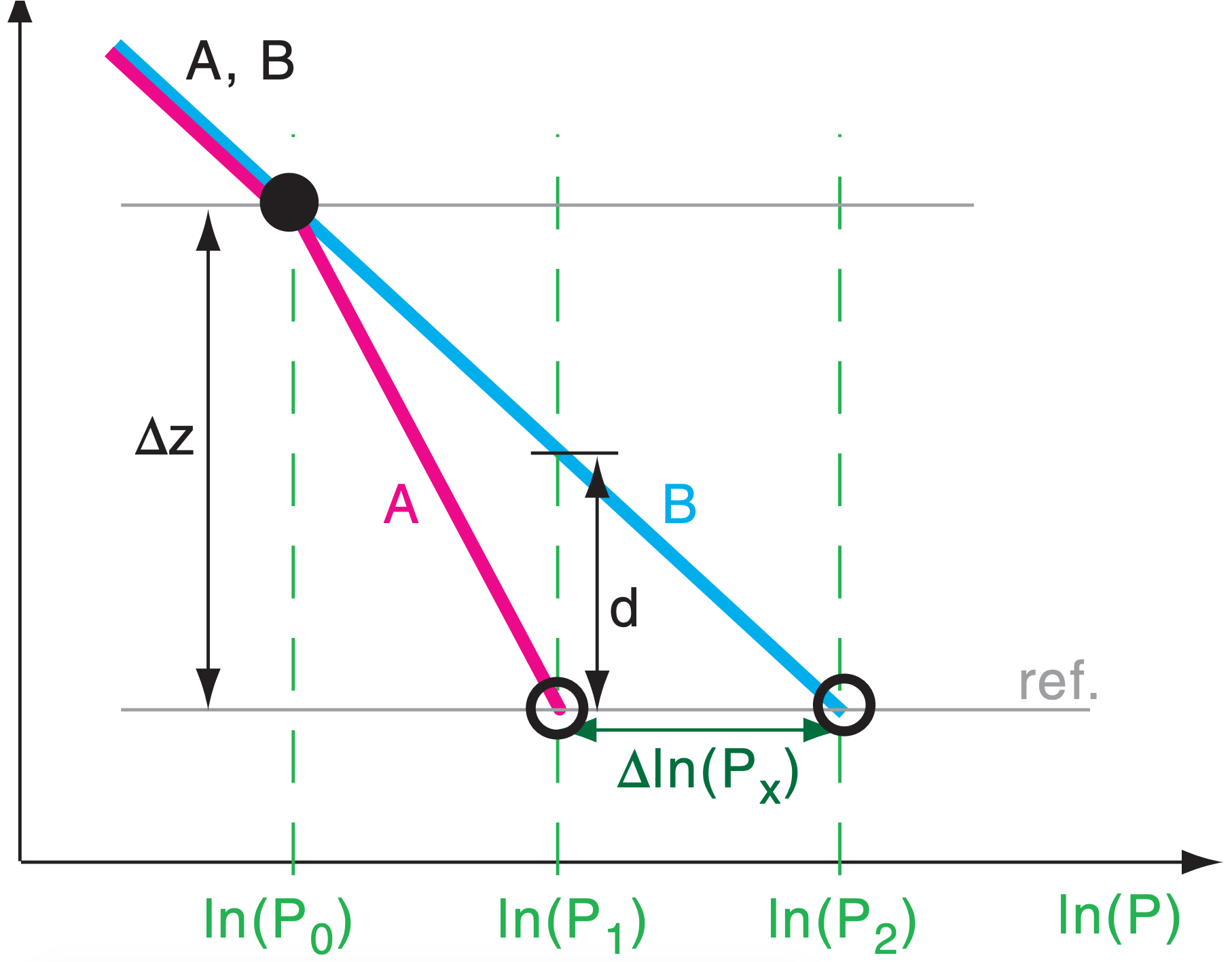
By the time you have descended distance ∆z from the black dot to the reference height, the pressure in the cold air has increased to P2, but in the warm air has increased a smaller amount to P1. Thus, at the reference height, there is a horizontal pressure difference ∆P = P2 – P1 pointing toward the mountain slope.
To quantify this effect, start with the hypsometric equation, separately for columns A and B:
Col. B at ref.: ln(P2) = ln(Po) + ∆z/(a·Te)
Col. A at ref: ln(P1) = ln(Po) + ∆z/(a·Tp)
where a = ℜd/|g| = 29.3 m K–1 from Chapter 1.
Subtract equation A from B
\(\ln \left(P_{2}\right)-\ln \left(P_{1}\right)=\dfrac{\Delta z}{a} \cdot\left(\dfrac{1}{T_{e}}-\dfrac{1}{T_{p}}\right)\)
Create a common denominator in the parentheses, and combine the ln() terms:
\(\ln \left(\dfrac{P_{2}}{P_{1}}\right)=\dfrac{\Delta z}{a} \cdot\left(\dfrac{T_{p}-T_{e}}{T_{e} \cdot T_{p}}\right)\)
Take the exponential of both sides, solve for P1:
\(P_{1}=P_{2} \cdot \exp \left(-\dfrac{\Delta z}{a} \cdot \dfrac{\Delta T}{T_{e}^{2}}\right)\)
where ∆T = Tp – Te , and where Te2 ≈ Te·Tp because both are absolute temperatures. Next, subtract P2 from both sides, and let ∆P = P1 – P2 be the pressure change in the positive x-direction at the reference height:
\(\Delta P=-P_{2} \cdot\left[1-\exp \left(-\dfrac{\Delta z}{a} \cdot \dfrac{\Delta T}{T_{e}^{2}}\right)\right]\)
Approximate the exponential with a truncated Taylor series: exp(–y) ≈ 1 – y + . . . Thus, the pressure decrease along the ref. height from B to A is
\(\ \begin{align} \Delta P \approx-P_{B} \cdot\left[\dfrac{\Delta z}{a} \cdot \dfrac{\Delta T}{T_{e}^{2}}\right]\tag{2}\end{align}\)
Expanding a and using the ideal gas law gives:
\(-\dfrac{\Delta P}{\rho} \approx|g| \cdot \Delta z \cdot \dfrac{\Delta T}{T_{e}}\)
Divide both sides by ∆x to give the horizontal pressure-gradient force per unit mass Fx PG/m :
\(\dfrac{F_{x P G}}{m}=-\dfrac{1}{\rho} \dfrac{\Delta P}{\Delta x}=|g| \cdot \dfrac{\Delta T}{T_{e}} \cdot \dfrac{\Delta z}{\Delta x}\)
Substituting ∆z/∆x = tan(α) gives the desired eq. (17.5), where α is the mountain slope angle.
\(\ \begin{align} \dfrac{F_{x P G}}{m}=-\dfrac{1}{\rho} \dfrac{\Delta P}{\Delta x}=|g| \dfrac{\Delta T}{T_{e}} \cdot \tan (\alpha)\tag{17.5}\end{align}\)
Also, in Fig. 17.c, d = z(P1 at B) – z(P1 at A) is the deflection distance of the near-mountain end of isobar P1 in Fig. 17.b.
To forecast the speed of the upslope flow, apply the equation of horizontal motion to a sloping surface and use eq. (17.6), which gives:
\(\ \begin{align} \dfrac{\Delta U_{s}}{\Delta t}=-U_{s} \dfrac{\Delta U_{s}}{\Delta s}-V \dfrac{\Delta U_{s}}{\Delta y}+|g| \dfrac{\Delta \theta_{v}}{T_{v e}} \sin (\alpha)+f_{c} \cdot V-C_{D} \dfrac{U_{s}^{2}}{\Delta z}\tag{17.7}\end{align}\)
\(\ tendency \quad\quad advection \quad\quad\quad buoyancy \quad\quad Coriolis\quad\quad drag \)
where Us is along-slope (up- or down-slope) flow, V is across-slope flow, ∆θv is virtual potential temperature difference between the slope-flow air and the environment (where ∆θv = ∆θ = ∆T for dry air), Tv is the absolute virtual temperature, fc = 2Ω·sin(latitude) is the Coriolis parameter, 2Ω = 1.458423x10⁻⁴ s–1, CD is a drag coefficient against the ground, and ∆z is the vertical depth of the slope flow.
Sample Application
For the scenario in the previous Sample Application, suppose a steady-state is reached where the only two forces are buoyancy and drag. Find the anabatic wind speed, assuming an anabatic flow depth of 50 m and drag coefficient of 0.05.
Find the Answer
Given: buoyancy term = 0.085 m·s–2 from previous Sample Application. CD = 0.05, ∆z = 50m
Find: Us = ? m s–1
Solve eq. (17.7) for Us, considering only buoyancy and drag terms:
Us = [(∆z/CD)·buoyancy term) ]1/2
= [ ((50m)/(0.05)) · (0.085 m·s–2) ]1/2 = 9.2 m s–1
Check: Units OK. Magnitude too large.
Exposition: In real anabatic flows, the temperature excess (5°C in this example) exists only close to the ground, and decreases to near zero by 50 to 100 m away from the mountain slope. If we had applied eq. (17.7) over the 5 m depth of the temperature excess, then a more-realistic answer of 2.9 m s–1 is found.
A better approach is to use the average temperature excess over the depth of the anabatic flow, not the maximum temperature excess measured close to the mountain slope.
Turbulence is strong during convective conditions such as during anabatic winds, which increases the turbulent drag against the ground.
17.3.2.2. Katabatic Wind
During anticyclonic conditions of calm or light synoptic-scale winds at night, air adjacent to a cold mountain slope can become colder than the surrounding air. This cold, dense air flows downhill under the influence of gravity (buoyancy), and is called a katabatic wind (Fig. 17.9). It can also form in the daytime over snow- or ice-covered slopes.
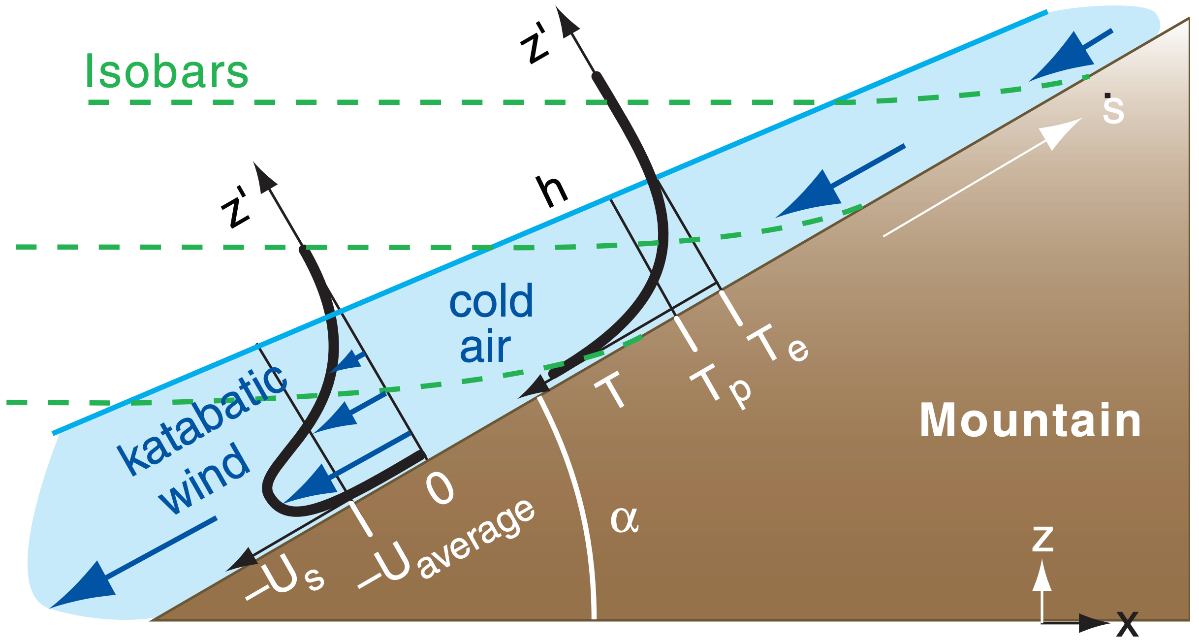
The katabatic wind is shallowest at the top of the slope, and increases in thickness and speed further downhill. Typical depths are 10 to 100 m, where the depth is roughly 5% of the vertical drop distance from the hill top. Typical speeds are 3 to 8 m s–1. Katabatic flows are shallower and less turbulent than anabatic flows.
Equation (17.7) also applies for katabatic flows, but with negative ∆θv. A horizontal pressure gradient drives the katabatic wind, but with hydrostatic air pressure increasing near the slope due to the cold dense air. Namely, isobars bend upward near the mountain during katabatic flows (Fig. 17.9).
The virtual potential temperature in a katabatic flow is generally coldest at the ground, and smoothly increases with height (Fig. 17.9). For the difference ∆θv = (θvp – θve), use the average temperature in the katabatic flow θvp minus the environmental temperature at the same altitude θve.
If there were no friction against the surface, then the fastest downslope winds would be where the air is the coldest; namely, closest to the ground. However, winds closest to the ground are slowed due to turbulent drag, leaving a nose of fast winds just above ground level (Fig. 17.9).
In Antarctica where downslope distances are hundreds of kilometers, the katabatic wind speeds are 3 to 20 m s–1 with extreme cases up to 50 m s–1, and durations of many days. These attributes are sufficiently large that Coriolis force turns the equilibrium wind direction 30 to 50° left of the fall line (a line pointing downhill). However, for most smaller valleys and slopes you can neglect Coriolis force and the across-slope (V) wind, allowing eq. (17.7) to be solved for some steady-state situations, as shown next.
Initially the wind (averaged over the depth of the katabatic flow) is influenced mostly by buoyancy and advection. It accelerates with distance s downslope:
\(\ \begin{align} \left|U_{\text {average}}\right|=\left[\left|g \cdot \dfrac{\Delta \theta_{v}}{T_{v e}} \cdot s \cdot \sin (\alpha)\right|\right]^{1 / 2}\tag{17.8}\end{align}\)
where |g| = 9.8 m·s–2, Tve is absolute temperature in the environment at the height of interest, α is the mountain slope angle, and s is distance downslope.
The average katabatic wind eventually approaches an equilibrium where drag balances buoyancy:
\(\ \begin{align} \left|u_{e q}\right|=\left[| g \cdot \dfrac{\Delta \theta_{v}}{T_{v e}} \cdot \dfrac{h}{C_{D}} \cdot \sin (\alpha)\right]^{1 / 2}\tag{17.9}\end{align}\)
where CD is the total drag against both the ground and the slower air aloft, and h is depth of the katabatic flow.
Sample Application (§)
Air adjacent to a 10° slope averages 10°C cooler over its 20 m depth than the surrounding air of virtual temperature 10°C. Find and plot the wind speed vs. downslope distance, and the equilibrium speed. CD = 0.005 .
Find the Answer
Given: ∆θv= –10°C, Tve=283 K, α= 10°, CD= 0.005
Find: U (m s–1) vs. x (km), where s ≈ x .
Use eq. (17.9) to find final equilibrium value:
\(\left|U_{e q}\right|=[| {\dfrac{\left(9.8 \mathrm{m} \cdot \mathrm{s}^{-2}\right) \cdot\left(-10^{\circ} \mathrm{C}\right)}{283 \mathrm{K}} \cdot \dfrac{(20 \mathrm{m})}{0.005} \cdot \sin \left(10^{\circ}\right)}|]^{1 / 2}\)
|Ueq| = 15.5 m s–1
Use eq. (17.8) for the initial variation.
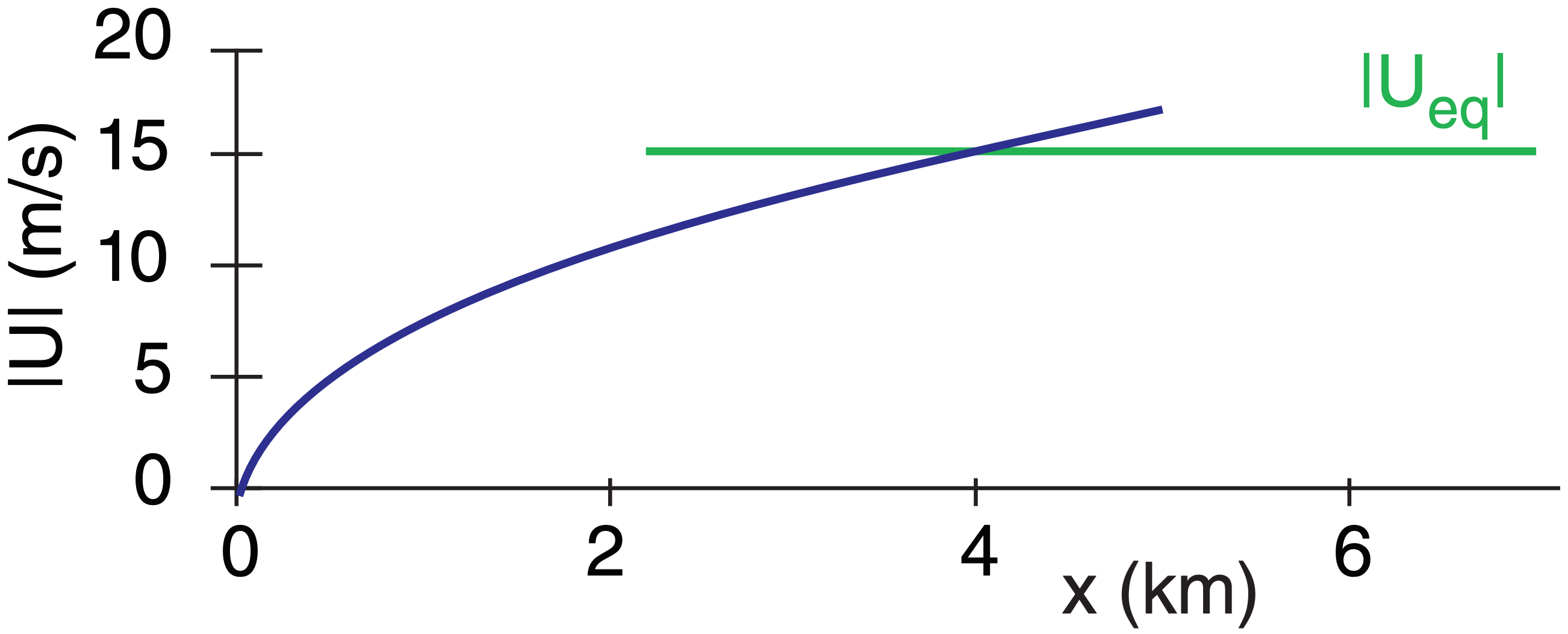
Check: Units OK. Physics OK.
Exposition: Although these two curves cross, the complete solution to eq. (17.7) smoothly transitions from the initial curve to the final equilibrium value.
17.3.3. Along-valley Winds
Katabatic and anabatic winds are part of larger circulations in the valley.
17.3.3.1. Night
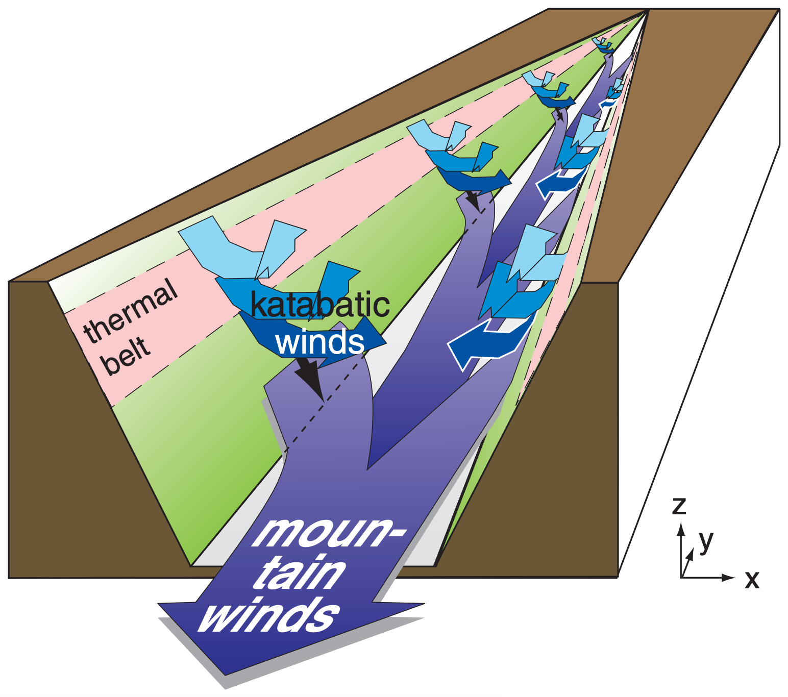
At night, the katabatic winds from the bottom of the slopes drain into the valley, where they start to accumulate. This pool of cold air is often stratified like a layer cake, with the coldest air at the bottom and less-cold air on top. Katabatic winds that start higher on the slope often do not travel all the way to the valley bottom (Fig. 17.10). Instead, they either spread out at an altitude where they have the same buoyancy as the stratified pool in the valley, or they end in a turbulent eddy higher above the valley floor. This leads to a relatively mild thermal belt of air at the mid to upper portions of the valley walls — a good place for vineyards and orchards because of fewer frost days.
Meanwhile, the cold pool of air in the valley bottom flows along the valley axis in the same direction that a stream of water would flow. As this cold air drains out of the valley onto the lowlands, it is known as a mountain wind. This is part of an along-valley circulation. A weak return flow aloft (not drawn), called the anti-mountain wind, flows up-valley, and is the other part of this alongvalley circulation.
17.3.3.2. Day
During anabatic conditions, there is often a weak cross-valley horizontal circulation (not drawn) from the tops of the anabatic updrafts back toward the center of the valley. Some of this air sinks (subsides) over the valley center, and helps trap air pollutants in the valley
During daytime, the upslope anabatic winds along the valley walls remove air from the valley floor. This lowers the pressure very slightly near the valley floor, which creates a pressure gradient that draws in replacement air from lower in the valley. These upstream flowing winds are called valley winds (Fig. 17.11), and are part of an along-valley circulation. A weak return flow aloft (heading down valley; not drawn in Fig. 17.11) is called the anti-valley wind.
17.3.3.3. Transitions
Because the sun angle relative to the mountain slope determines the solar heating rate of that slope, the anabatic winds on one side of the valley are often stronger than on the other. At low sun angles near sunrise or sunset, the sunny side of the valley might have anabatic winds while the shady side might have katabatic winds.
17.3.4. Sea breeze
A sea breeze is a shallow cool wind that blows onshore (from sea to land) during daytime (Fig. 17.12). It occurs in large-scale high-pressure regions of weak or calm geostrophic wind under mostly clear skies. Similar flows called lake breezes form along lake shorelines, and inland sea breezes form along boundaries between adjacent land regions with different land-use characteristics (e.g., irrigated fields of crops adjacent to drier land with less vegetation).
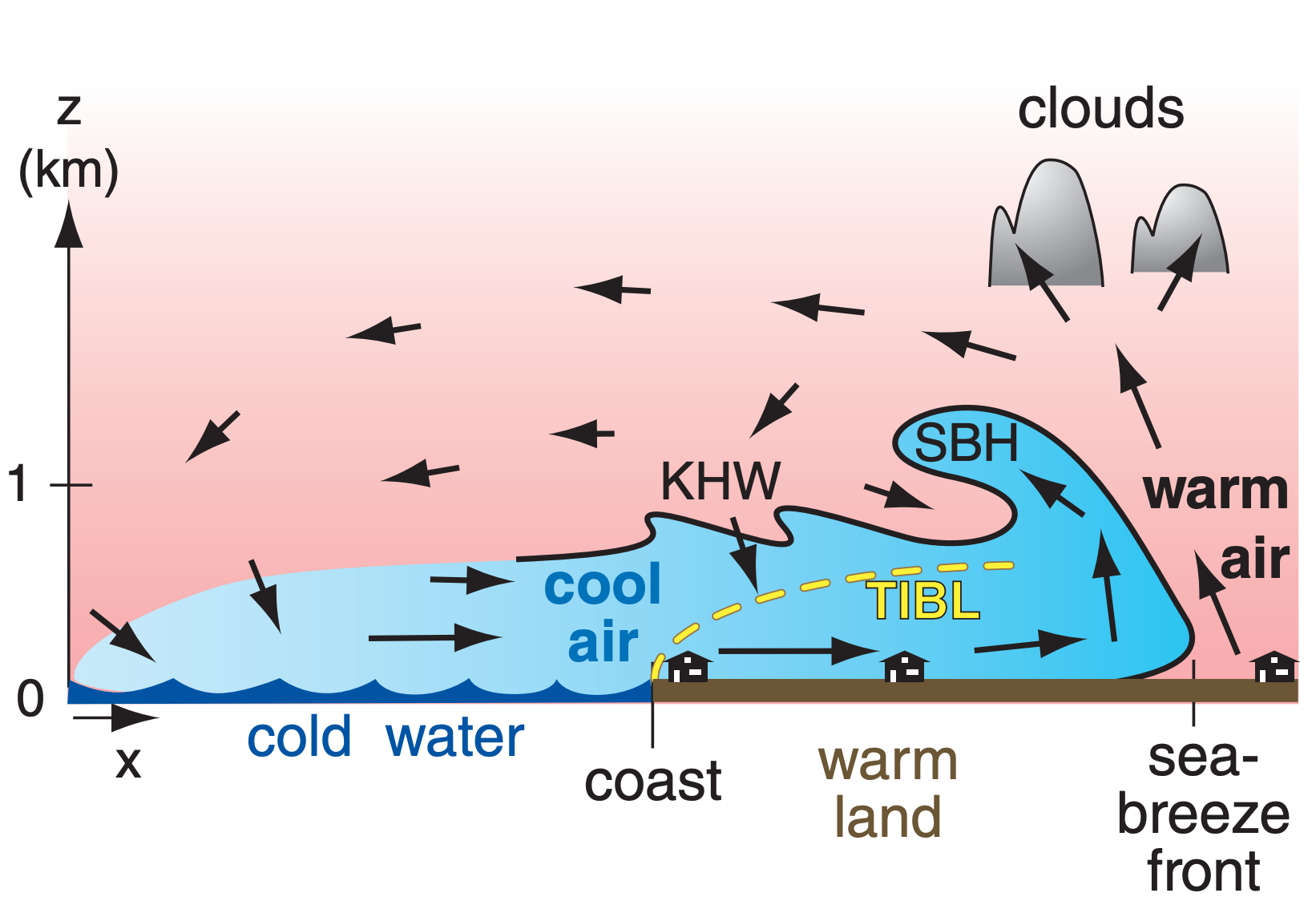
The sea breeze is caused by a 5 °C or greater temperature difference between the sun-heated warm land and the cooler water. It is a surface manifestation of a thermally driven mesoscale circulation called the sea-breeze circulation, which often includes a weak return flow aloft from land to sea.
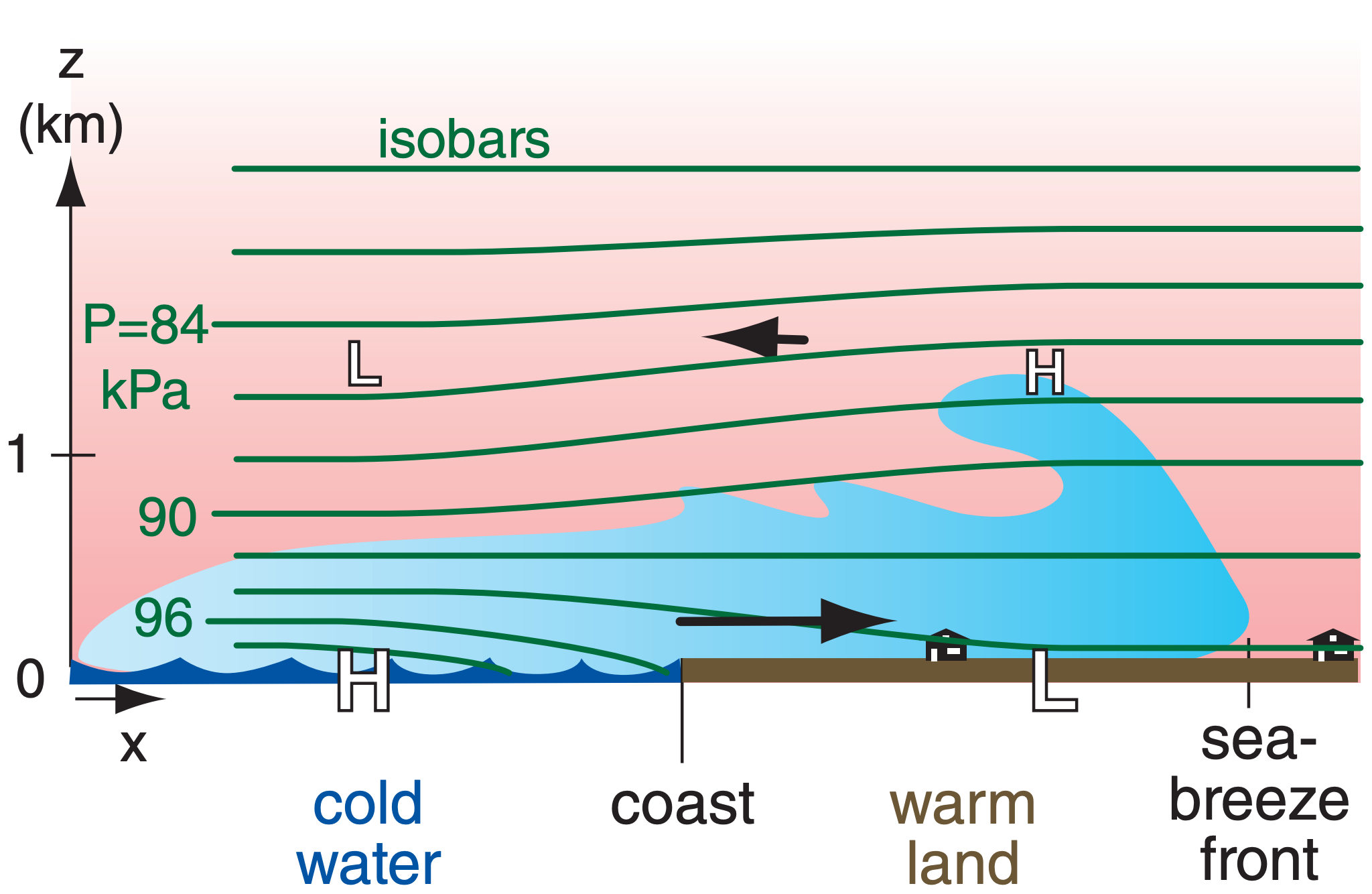
For warm air over land, the hypsometric equation states that hydrostatic pressure does not decrease as rapidly with increasing height as it does in the cooler air over the sea (Fig. 17.13). This creates a pressure gradient aloft between higher pressure over land and lower pressure over the sea, which initiates a wind aloft. This wind moves air molecules from over land to over sea, causing surface pressure over the warm land to decrease because fewer total molecules in the warm-air column cause less weight of air at the base of the column. Similarly, the surface pressure over the water increases due to molecules added to the cool-air column. This creates a pressure gradient near the surface that drives the bottom portion of the sea-breeze circulation. Such hydrostatic thermal circulations were explained in the General Circulation chapter.
A sea-breeze front marks the leading edge of the advancing cool marine air and behaves similarly to a weak advancing cold front or a thunderstorm gust front. If the updraft ahead of the front is humid enough, a line of cumulus clouds can form along the front, which can grow into a line of thunderstorms if the atmosphere is convectively unstable.
The raised portion of cool air immediately behind the front, called the sea-breeze head, is analogous to the head at the leading edge of a gust front. The sea-breeze head is roughly twice as thick as the subsequent portion of the feeder cool onshore flow (which is 0.5 to 1 km thick). The top of the seabreeze head often curls back in a large horizontal roll eddy over warmer air from aloft.
Vertical wind shear at the density interface between the low-level sea breeze and the return flow aloft can create Kelvin-Helmholtz (KH) waves. These breaking waves in the air have wavelength of 0.5 to 1 km. The KH waves increase turbulent drag on the sea breeze by entraining low-momentum air from above the interface. A slowly subsiding return flow occurs over water and completes the circulation as the air is again cooled as it blows landward over the cold water.
As the cool marine air flows over the land, a thermal internal boundary layer (TIBL) forms just above the ground (Fig. 17.12). The TIBL grows in depth zi with the square root of distance x from the shore as the marine air is modified by the heat flux FH (in kinematic units K·m s–1) from the underlying warm ground:
\(\ \begin{align} z_{i}=\left[\dfrac{2 \cdot F_{H}}{\gamma \cdot M} \cdot x\right]^{1 / 2}\tag{17.10}\end{align}\)
where γ = ∆θ/∆z is the gradient of potential temperature in the air just before reaching the coast, and M is the wind speed.
Sample Application
What horizontal pressure difference is needed in the bottom part of the sea-breeze circulation to drive a onshore wind that accelerates from 0 to 6 m s–1 in 6 h?
Find the Answer
Given: ∆M/∆t = (6 m s–1)/(6 h) = 0.000278 m·s–2
Find: ∆P/∆x = ? kPa km–1
Neglect all other terms in the horiz. eq. of motion:
\( \begin{align} \Delta M / \Delta t=-(1 / \rho) \cdot \Delta P / \Delta x\tag{10.23a}\end{align}\)
Assume air density is ρ = 1.225 kg m–3 at sea level.
Solve for ∆P/∆x :
∆P/∆x = –ρ · (∆M/∆t) = –(1.225kg m–3)·(0.000278m·s–2)
= –0.00034 kg·m–1·s–2/m = –0.00034 Pa m–1
= –0.00034 kPa km–1
Check: Units OK. Magnitude OK.
Exposition: Only a small pressure gradient is needed to drive a sea breeze.
Sample Application
For a surface kinematic heat flux of 0.2 K m s–1, wind speed of 5 m s–1, and γ = 3K km–1, find the TIBL depth 5 km from shore.
Find the Answer
Given: FH=0.2 K·m s–1, M=5 m s–1, γ =3K km–1, x=5 km
Find: zi = ? m
Use eq. (17.10):
zi = [2·(0.2K·m s–1)·(5km) / {(3K km–1)·(5m s–1)} ]1/2 = 0.365 km
Check: Units OK. Magnitude reasonable.
Exposition: Above this height, the air still feels the marine influence, and not the warmer land.
In early morning, the sea-breeze circulation does not extend very far from the coast, but advances further over land and water as the day progresses. Advancing cold air behind the sea-breeze front behaves somewhat like a density current or gravity current in which a dense fluid spreads out horizontally beneath a less dense fluid. When this is simulated in water tanks, the speed MSBF of advance of the sea-breeze front, is
\(\ \begin{align} M_{S B F}=k \cdot \sqrt{|g| \cdot \dfrac{\Delta \theta_{v}}{T_{v}} \cdot d}\tag{17.11}\end{align}\)
where ∆θv is the virtual potential temperature difference between the cool marine sea-breeze air and the warmer air over land that is being displaced, Tv is an absolute average virtual temperature, |g| = 9.8 m·s–2 is gravitational acceleration magnitude, d is depth of the density current, and constant k ≈ 0.62 .
When fully developed, surface (10 m height) wind speeds in the marine, inflow portion of the sea breeze at the coast are 1 to 10 m s–1 with typical values of 6 m s–1. The relationship between seabreeze wind speed M at the coast and speed of the sea-breeze front is:
\(\ \begin{align} M \approx 1.15 \cdot M_{S B F}\tag{17.12}\end{align}\)
Sample Application
Marine-air of thickness 500 m and virtual temperature 16°C is advancing over land. The displaced continental-air virtual temperature is 20°C. Find the seabreeze front speed, and the sea-breeze wind speed.
Find the Answer
Given: ∆θv = ∆Tv = 20 – 16°C = 4°C , d = 500 m, Tv average = (16+20°C)/2 = 18°C = 291K
Find: MSBF = ? m s–1, M = ? m s–1
For speed-of-advance of the front, use eq. (17.11):
MSBF = (0.62) · [(9.8m·s–2)·(4K)·(500m)/(291K)]1/2 = 5.1 m s–1
For the sea-breeze wind speed, use eq. (17.12):
M = 1.15 · (5.1m s–1) = 5.9 m s–1
Check: Units OK. Magnitude OK.
Exposition: Because the sea-breeze circulation extends 20 to 250 km over the sea, mariners used these reliable breezes to sail north-south along the Atlantic coasts of Europe and Africa centuries ago. Upon reaching the latitude of the easterly trade winds in the tropical global circulation, they then sailed west towards the Americas. Upon reaching the Americas, they again used the sea-breezes to sail north and south along the East Coasts of North and South America. For the return trip to Europe, they sailed in the mid-latitude westerlies. Thus, by using both local sea-breeze winds and the global circulation, they achieved an effective commercial trade route.
The sea-breeze front can advance L = 10 to 200 km inland by the end of the day, although typical advances are L = 20 to 60 km unless inhibited by mountains or by opposing synoptic-scale winds. Even without mountain barriers, the sea breeze will eventually turn away from its advance due to Coriolis force. For latitudes ≠ 30° (to avoid a divide-by-zero error), L is roughly
\(\ \begin{align} L \approx \dfrac{M_{S B F}}{\left|\omega^{2}-f_{c}^{2}\right|^{1 / 2}}\tag{17.13}\end{align}\)
where MSBF is given by the previous equation, ω = 2π day–1 = 7.27x10⁻⁵ s–1 is the frequency of the daily heating/cooling cycle, and fc = (1.458x10⁻⁴ s–1)·sin(latitude) is the Coriolis parameter. As the front advances, prefrontal waves may cause wind shifts ahead of the front.
Sample Application
Assuming calm synoptic conditions (i.e., no largescale winds that oppose or enhance the sea-breeze), what maximum distance inland would a sea-breeze propagate. Use data from the previous Sample Application, for a latitude of 45°N.
Find the Answer
Given: MSBF = 5.1 m s–1 from previous example. latitude = 45°N.
Find: L = ? km
First, find the Coriolis parameter:
fc = (1.458x10⁻⁴ s–1)·sin(45°) = 1.03x10⁻⁴ s–1
Use eq. (17.13):
L = (5.1 m s–1) / [(7.27x10⁻⁵ s–1)2 – (1.03x10⁻⁴ s–1)2] 1/2 = 70 km
Check: Units OK. Magnitude reasonable.
Exposition: At 30° latitude the denominator of eq. (17.13) is zero, causing L = ∞. But this is physically unreasonable. Thus, we expect eq. (17.13) to not be reliable at latitudes near 30°.
At the end of the day, the sea-breeze circulation dissipates and a weaker, reverse circulation called the land-breeze forms in response to the nighttime cooling of the land surface relative to the sea. Sometimes, the now-disconnected sea-breeze front from late afternoon continues to advance farther inland during the night as a bore (the front of dense fluid advancing under less-dense fluid; also described as a propagating solitary wave with characteristics similar to the hydraulic jump). In Australia, such a bore and its associated cloud along the wave crest are known as the Morning Glory.
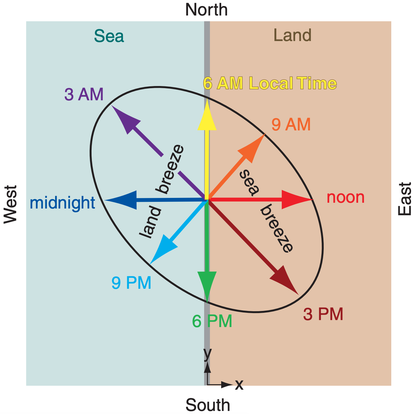
In the vertical cross section normal to the coastline (as in Fig. 17.12), the surface wind oscillates back and forth between onshore and offshore, reversing directions during the morning and evening hours. The Coriolis force induces an oscillating along-shore wind component that lags the onshore-offshore component by 6 h (or 1/4 of a daily cycle). Hence, the horizontal wind vector rotates throughout the course of the day. Rotation is clockwise in the northern hemisphere and counterclockwise in the southern hemisphere.
The idealized sea-breeze hodograph has an elliptical shape (Fig. 17.14). For example, along a meridional coastline with the ocean to the west in the Northern Hemisphere, the diurnal component of the surface wind tends to be westerly (onshore) during the mid-day, northerly (alongshore) during the evening, easterly near midnight, and southerly (alongshore) near sunrise.
The sea-breeze wind and the mean (24 h average) synoptic-scale surface wind are additive. If the synoptic-scale wind in the above example is blowing from the north, the surface wind speed will tend to be higher around sunset when the mean wind and the diurnal component are in the same direction, than around sunrise when they oppose each other.
Many coasts have complex shaped coastlines with bays or mountains, resulting in a myriad of interactions between local flows that distort the sea breeze and create regions of enhanced convergence and divergence. The sea breeze can also interact with boundary-layer thermals, and urban circulations, causing complex dispersion of pollutants emitted near the shore. If the onshore synoptic-scale geostrophic wind is too strong, only a TIBL develops with no sea-breeze circulation.
In regions such as the west coast of the Americas, where major mountain ranges lie within a few hundred kilometers of the coast, sea breezes and terraininduced winds appear in combination.