12.1.14: Routine X-Ray Analysis- Powder Diffraction

Figure 12.20: A powder diffractometer

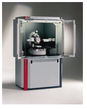
Mineralogists use two fundamental X-ray diffraction techniques: powder diffraction and single-crystal diffraction. Powder diffraction is much more common; we use it for routine mineral identification and for determining unit cell dimensions. We can also sometimes use this technique to learn the proportions of different minerals in a rock or other mineral mixture. Single crystal diffraction, on the other hand, provides information necessary for determining a crystal’s space group and the arrangement of atoms in a crystal’s unit cell. We do not normally use powder diffraction to figure out atomic arrangements in crystals because powder diffraction data are more ambiguous for this purpose than single crystal data. Different X-ray peaks correspond to different crystals in the powdered sample, and the data do not reveal the orientations of crystals or planes causing diffraction. The Rietveld method, an extension of normal powder diffraction analysis, sometimes overcomes these complications.

For now, we will focus our discussion on powder diffraction and return to single-crystal techniques later. Figure 12.20 shows a typical powder diffractometer. The cabinet is about 2 meters tall.

Figure 12.21: A sample holder being loaded with a powdered sample

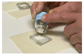
To prepare a sample for powder diffraction, we grind it to a fine powder. The goal is to have a near-infinite number of fine crystallites in random orientations. We load the powder into holders, such as the one in Figure 12.21 or put it on a glass slide. When lots of crystals in different orientations are X-rayed, many crystals will satisfy Bragg’s law for every set of (hkl) planes. Thus, when an X-ray beam hits the sample, hundreds or thousands of diffracted beams will go in different directions. Some diffracted beams will have high intensity and others will have medium or low intensity.

Figure 12.22: Diffraction cones

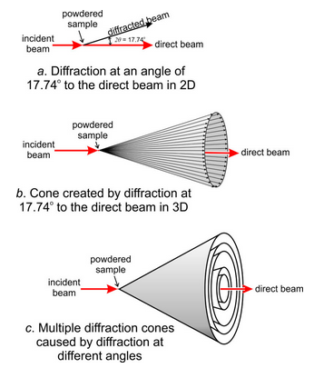
Consider a powdered sample of some mineral with (111) planes having a d-value of 5.0 Å. For Cu Kα, then, Bragg’s Law tells us this will cause diffraction at a 2θ angle of 17.74°. When we X-ray the sample, many crystals will be oriented to cause diffraction at 17.74° to the incident X-ray beam. Figure 12.22a shows this in two dimensions. But, diffraction can go in any direction at 17.74° to the beam and, consequently, diffracted beams create a diffraction cone in three dimensions (Figure 12.22b)

In most crystals, a large number of d-values cause measurable diffraction. Each produces a cone at a different 2θ angle to the X-ray beam. Figure 12.22c shows a small number of cones corresponding to different d-values – minerals typically produce many more than shown here. The cones are all concentric with the direct X-ray beam.

Figure 12.23: X-ray diffraction geometry and a modern diffractometer

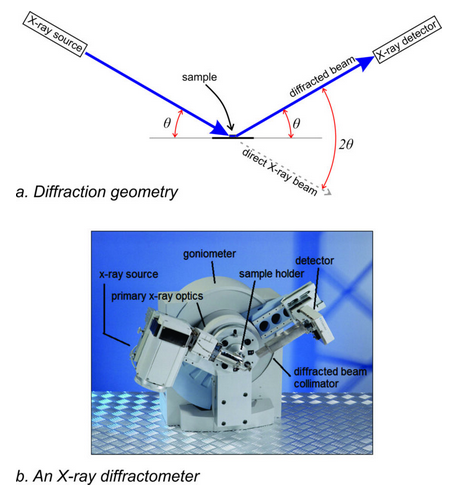
Because we powdered the sample and get diffraction cones instead of separate rays going in discreet directions, we do not have to measure angles and intensities in 3D space. Some diffractometers are slightly different, but Figure 12.23a shows the basic geometry of diffraction. The photo in Figure 12.23b shows a modern diffractometer with this geometry. Besides an X-ray source (tube) and a detector (which measures the intensity of diffracted X-ray beams), the device includes several collimators and filters that enhance analysis.

In most diffractometers, the sample is at a fixed location (although it may be rotated by a device called a goniometer). The tube and detector, move in a planar circular arc, usually vertically, to measure diffraction intensities for 2θ values from very low angles to some high value. In practice, most diffractometers cannot measure peaks at angles below 1 or 2° 2θ because the direct X-ray beam bombards the detector. The upper 2θ limit of measurement usually depends on the need of the mineralogist, but for most purposes we do not need data above 60° to 70° 2θ.

During analysis, the incident X-ray beam strikes the sample at many different θ angles while the detector moves to maintain Bragg Law (reflection) geometry. The angle of incidence and the angle of reflection are the same, so after being diffracted an X-ray beam travels at an angle of 2θ from the incident beam. Because a crystal contains many differently spaced atoms, diffraction occurs at many 2θ angles.

If a diffracted beam is to hit the detector, two requirements must be met:

• A family of planes with d_hkl must be oriented at an angle (θ) to the incident beam that satisfies Bragg’s Law.
• The detector must be at the correct angle (2θ) from the incident beam to intercept the diffracted X-rays.

Because the angle between the detector and the X-ray beam is 2θ, mineralogists usually report X-ray results as peak intensities for different 2θ values. For example, reference books list the two most intense diffraction peaks of fluorite (using Cu Kα radiation) as 28.3° and 47.4° 2θ. We must remember to divide 2θ values by 2 before we use them with Bragg’s Law to calculate d-values.