60.7: Examples to help train your eye
- Page ID
- 22865
\( \newcommand{\vecs}[1]{\overset { \scriptstyle \rightharpoonup} {\mathbf{#1}} } \)
\( \newcommand{\vecd}[1]{\overset{-\!-\!\rightharpoonup}{\vphantom{a}\smash {#1}}} \)
\( \newcommand{\id}{\mathrm{id}}\) \( \newcommand{\Span}{\mathrm{span}}\)
( \newcommand{\kernel}{\mathrm{null}\,}\) \( \newcommand{\range}{\mathrm{range}\,}\)
\( \newcommand{\RealPart}{\mathrm{Re}}\) \( \newcommand{\ImaginaryPart}{\mathrm{Im}}\)
\( \newcommand{\Argument}{\mathrm{Arg}}\) \( \newcommand{\norm}[1]{\| #1 \|}\)
\( \newcommand{\inner}[2]{\langle #1, #2 \rangle}\)
\( \newcommand{\Span}{\mathrm{span}}\)
\( \newcommand{\id}{\mathrm{id}}\)
\( \newcommand{\Span}{\mathrm{span}}\)
\( \newcommand{\kernel}{\mathrm{null}\,}\)
\( \newcommand{\range}{\mathrm{range}\,}\)
\( \newcommand{\RealPart}{\mathrm{Re}}\)
\( \newcommand{\ImaginaryPart}{\mathrm{Im}}\)
\( \newcommand{\Argument}{\mathrm{Arg}}\)
\( \newcommand{\norm}[1]{\| #1 \|}\)
\( \newcommand{\inner}[2]{\langle #1, #2 \rangle}\)
\( \newcommand{\Span}{\mathrm{span}}\) \( \newcommand{\AA}{\unicode[.8,0]{x212B}}\)
\( \newcommand{\vectorA}[1]{\vec{#1}} % arrow\)
\( \newcommand{\vectorAt}[1]{\vec{\text{#1}}} % arrow\)
\( \newcommand{\vectorB}[1]{\overset { \scriptstyle \rightharpoonup} {\mathbf{#1}} } \)
\( \newcommand{\vectorC}[1]{\textbf{#1}} \)
\( \newcommand{\vectorD}[1]{\overrightarrow{#1}} \)
\( \newcommand{\vectorDt}[1]{\overrightarrow{\text{#1}}} \)
\( \newcommand{\vectE}[1]{\overset{-\!-\!\rightharpoonup}{\vphantom{a}\smash{\mathbf {#1}}}} \)
\( \newcommand{\vecs}[1]{\overset { \scriptstyle \rightharpoonup} {\mathbf{#1}} } \)
\( \newcommand{\vecd}[1]{\overset{-\!-\!\rightharpoonup}{\vphantom{a}\smash {#1}}} \)
\(\newcommand{\avec}{\mathbf a}\) \(\newcommand{\bvec}{\mathbf b}\) \(\newcommand{\cvec}{\mathbf c}\) \(\newcommand{\dvec}{\mathbf d}\) \(\newcommand{\dtil}{\widetilde{\mathbf d}}\) \(\newcommand{\evec}{\mathbf e}\) \(\newcommand{\fvec}{\mathbf f}\) \(\newcommand{\nvec}{\mathbf n}\) \(\newcommand{\pvec}{\mathbf p}\) \(\newcommand{\qvec}{\mathbf q}\) \(\newcommand{\svec}{\mathbf s}\) \(\newcommand{\tvec}{\mathbf t}\) \(\newcommand{\uvec}{\mathbf u}\) \(\newcommand{\vvec}{\mathbf v}\) \(\newcommand{\wvec}{\mathbf w}\) \(\newcommand{\xvec}{\mathbf x}\) \(\newcommand{\yvec}{\mathbf y}\) \(\newcommand{\zvec}{\mathbf z}\) \(\newcommand{\rvec}{\mathbf r}\) \(\newcommand{\mvec}{\mathbf m}\) \(\newcommand{\zerovec}{\mathbf 0}\) \(\newcommand{\onevec}{\mathbf 1}\) \(\newcommand{\real}{\mathbb R}\) \(\newcommand{\twovec}[2]{\left[\begin{array}{r}#1 \\ #2 \end{array}\right]}\) \(\newcommand{\ctwovec}[2]{\left[\begin{array}{c}#1 \\ #2 \end{array}\right]}\) \(\newcommand{\threevec}[3]{\left[\begin{array}{r}#1 \\ #2 \\ #3 \end{array}\right]}\) \(\newcommand{\cthreevec}[3]{\left[\begin{array}{c}#1 \\ #2 \\ #3 \end{array}\right]}\) \(\newcommand{\fourvec}[4]{\left[\begin{array}{r}#1 \\ #2 \\ #3 \\ #4 \end{array}\right]}\) \(\newcommand{\cfourvec}[4]{\left[\begin{array}{c}#1 \\ #2 \\ #3 \\ #4 \end{array}\right]}\) \(\newcommand{\fivevec}[5]{\left[\begin{array}{r}#1 \\ #2 \\ #3 \\ #4 \\ #5 \\ \end{array}\right]}\) \(\newcommand{\cfivevec}[5]{\left[\begin{array}{c}#1 \\ #2 \\ #3 \\ #4 \\ #5 \\ \end{array}\right]}\) \(\newcommand{\mattwo}[4]{\left[\begin{array}{rr}#1 \amp #2 \\ #3 \amp #4 \\ \end{array}\right]}\) \(\newcommand{\laspan}[1]{\text{Span}\{#1\}}\) \(\newcommand{\bcal}{\cal B}\) \(\newcommand{\ccal}{\cal C}\) \(\newcommand{\scal}{\cal S}\) \(\newcommand{\wcal}{\cal W}\) \(\newcommand{\ecal}{\cal E}\) \(\newcommand{\coords}[2]{\left\{#1\right\}_{#2}}\) \(\newcommand{\gray}[1]{\color{gray}{#1}}\) \(\newcommand{\lgray}[1]{\color{lightgray}{#1}}\) \(\newcommand{\rank}{\operatorname{rank}}\) \(\newcommand{\row}{\text{Row}}\) \(\newcommand{\col}{\text{Col}}\) \(\renewcommand{\row}{\text{Row}}\) \(\newcommand{\nul}{\text{Nul}}\) \(\newcommand{\var}{\text{Var}}\) \(\newcommand{\corr}{\text{corr}}\) \(\newcommand{\len}[1]{\left|#1\right|}\) \(\newcommand{\bbar}{\overline{\bvec}}\) \(\newcommand{\bhat}{\widehat{\bvec}}\) \(\newcommand{\bperp}{\bvec^\perp}\) \(\newcommand{\xhat}{\widehat{\xvec}}\) \(\newcommand{\vhat}{\widehat{\vvec}}\) \(\newcommand{\uhat}{\widehat{\uvec}}\) \(\newcommand{\what}{\widehat{\wvec}}\) \(\newcommand{\Sighat}{\widehat{\Sigma}}\) \(\newcommand{\lt}{<}\) \(\newcommand{\gt}{>}\) \(\newcommand{\amp}{&}\) \(\definecolor{fillinmathshade}{gray}{0.9}\)When strata are horizontal, you only see the top layer unless erosion has cut down through it (in stream channels, say), exposing deeper layers. The overall pattern is that the geologic contacts follow the contour lines, and don’t vary much in elevation. In areas of dendritic drainage, such as the Atlantic Coastal Plain, the Great Plains, or the Colorado Plateau, this produces a distinctive branching pattern to the geologic map, as in these two examples:
Angular unconformities are as distinctive on geologic maps as they are in cross-section: two sets of formations meet each other at an abrupt angle. The lower, older formations will typically be folded or tilted, while the upper, younger formations will typically be close to horizontal.
So how do you recognize anticlines vs. synclines on geologic maps? There are two main techniques: (1) look for strike and dip symbols, and (2) look for age patterns. In an anticline, the strata dip outward away from the axis (hinge) of the fold. The anticline’s oldest strata will appear in the middle, and younger strata will appear on the limbs. In a syncline, the strata dip inward toward the axis (hinge) of the fold. The syncline’s youngest strata will appear in the middle, and older strata will appear on the limbs.

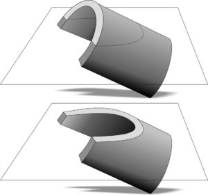
When a fold plunges into the Earth at some angle, its outcrop pattern changes from a series of parallel stripes to a series of nested “V” shapes. As with non-plunging folds (those that have horizontal hinges), in a plunging anticline, the oldest strata are in the middle, and the strata dip outward on the two limbs. And as with a with non-plunging synclines, plunging synclines also have the oldest strata on the limbs, and the strata dip inward toward the youngest strata in the middle.
In this example, you can tell it’s an anticline, because it has older strata in the middle (Devonian, D) and younger strata on the limbs (Mississippian and Pennsylvanian, M and PP):
In contrast, here (same map, different fold), you can see the pattern is reversed. This allows you to deduce that it’s a syncline, because Mississippian strata are the middle (younger) and Devonian and Silurian strata occur on the limbs of the fold (older).
In this example, you can see the strike and dip symbols more or less parallel to the contacts between the beds, and dipping westward on the west limb, and eastward on the east limb. This tells you it must be an anticline:
Here are two examples showing normal faults...
The first one is marked with D/U notation showing which side went down and which went up:
...And this one shows the alternate style, with a little dip-tick coming off the fault trace, on the down-dropped side. Sometimes, as with this example, the mapmaker puts a little “ball” at the end of the tick-mark, making it look like a lollypop:
With thrust faults, a saw-toothed pattern is used. The little triangular “teeth” are on the upper block of rock. There are a lot of examples in this map!
Unlike anticlines and synclines, structural domes and basins are areas where the strata are flexed around a central point, rather than a line (fold axis or hinge). In map view, they appear like “bull’s eyes” with a series of concentric rings of strata. If the strata dip outward away from that central point, then it is a structural dome. Structural domes expose their oldest strata in their center, while strata get younger toward the outer edges of the structure. The reverse is true for structural basins: they are structurally lowest in the middle, so all the strata dip inward toward that “deepest” part of the structure. This means that structural basins expose their youngest strata in their center, while strata get older toward the outer edges of the structure.
Here is an example from Utah: the San Rafael Swell is a structural dome. If you zoom in, you’ll see the pale blue strata exposed in the middle are Permian, with strata getting younger (Triassic, then Jurassic, and then Cretaceous) as you work your way outward toward the edges.
Another example, of the opposite situation: here, in northern New Mexico, is a structural basin, with the youngest strata (Tsj) is surrounded by progressively older and older strata (Tn, Toa), into the Cretaceous series (they start with K):
As a friendly reminder, the 1746 Guettard / Buache map of the chalk outcrops around the Paris Basin was another example of a structural basin.
Now that we’ve covered these basics, it’s time to test yourself...


