39.1: A Quaternary Quandary

Our modern geologic periods, epochs, and ages have been a state of flux. Currently, we live in the Meghalayan Age of the Holocene Epoch of the Quaternary Period of the Cenozoic Era of the Phanerozoic Eon. However, there have been many changes to this hierarchy over the last few hundred years, with significant changes recently.

Figure \(\PageIndex{1}\): Giovanni Arduino (Source: CC BY 4.0; By Istituto Veneto di Scienze, Lettere ed Arti, https://commons.wikimedia.org/w/inde...curid=38573367).

Our modern sense of geologic time began in northern Italy. In 1759, a man by the name of Giovanni Arduino introduced three terms to help make sense of the geology of the Alps where he worked. He used the term “Primary” for the ancient metamorphic cores of the mountains, “Secondary” for the hard sedimentary rocks on the flanks, and “Tertiary” for the sedimentary rocks in the foothills, which were not quite as hard. Primary and Secondary were eventually dropped by scientists because they did not always describe what was seen in regions in other areas. Tertiary remained. In 1829, French geologist Jules Desnoyers added the term “Quaternary” to describe the most recent geological materials, including lava flows and loose sediments. The terms Tertiary and Quaternary are still with us, though embattled in different ways, their dates and how they are viewed having changed over time. As recently as 2000, these two periods comprised the entire Cenozoic Era, with the Tertiary Period lasting from 65 Ma until 2.58 Ma and the Quaternary Period running from 2.58 Ma to the present.

Figure \(\PageIndex{2}\): The Cenozoic Era. The Tertiary Period has been formally removed and the Paleogene and Neogene made Periods. This chart reflects the former situation prior to these changes (Source: The Geological Society).

In 2004, the keepers of geologic time, the ICS (International Commission on Stratigraphy) completely dropped the terms Tertiary and Quaternary from the time scale, replacing them with two divisions, the Paleogene Period (66 Ma to 23 Ma) and the Neogene Period (23 Ma to 2.58 Ma). This was done in order to standardize the Cenozoic Era time periods to be consistent with the rest of the time scale. Marine geologists felt that the Neogene should also encompass all of the most recent portions of time. A major disagreement arose, however, because terrestrial geologists felt that the most recent geological materials on land required that the old term Quaternary Period be retained. These sediments and formations included all of the ice age materials, which are different from Neogene materials prior to 2.58 Ma. Terrestrial workers won the argument and in 2009, the ICS voted to reinstate the Quaternary Period.

The base of the the Quaternary is marked by the beginning of what is known as the Gelasian Stage. The lower boundary of this chronostratigraphic unit is marked by a GSSP location near Gela, Italy, and is primarily a magnetostratigraphic boundary, but secondarily marks the extinction of a number of calcareous nanofossils. Perhaps most importantly, the Gelasian Age (“Stage” is a chronostratigraphic term equivalent to the lithostratigraphic term “Age”) marks the start of the growth of northern hemisphere glaciers and ice sheets. You may know this time by another name: the Pleistocene Epoch. Perhaps images of mammoth, mastodon, saber-toothed cats, and early humans perhaps just popped into your mind!

Currently, the Quaternary Period is broken up into two Epochs, the Pleistocene Epoch (2.58 Ma to 11.7 Ka) and the Holocene Epoch. There is a move to add another time division, something perhaps called “Anthropocene,” but it is not finalized yet. We will come back to that later.

Did I Get It? - Quiz

Exercise \(\PageIndex{1}\)

Geologic "Periods", like the Quaternary Period, are not necessarily static. What are some of the characteristics of a unit of geologic time that cannot change as new information arises?

a. Fossils that define the period

b. End dates

c. Name

d. Anything can change with new information

Answer

d. Anything can change with new information

MARINE ISOTOPIC STAGES: DEFINING THE PLEISTOCENE AND HOLOCENE EPOCHS

Figure \(\PageIndex{3}\): Sections of sedimentary deep sea cores from off the coast of Greenland (Source: CC BY 3.0; By Hannes Grobe (talk) – Own work, https://commons.wikimedia.org/w/inde...?curid=6829604).

The Quaternary Period differs from the Paleogene and Neogene Periods because it is defined by ice age cycles, known as greenhouse (interglacial) and icehouse (glacial) periods. An entire glacial/interglacial cycle typically lasts about 100,000 years and is driven by Milankovitch orbital changes. And, there are enough of these that the record is quite complicated. When you look at the climate record of the Pleistocene Epoch, however, you see many, many more up and down swings in temperature. These smaller, or shorter, changes in temperature during a glacial period are “stadials” and “interstadials”.

In addition to ice cores, researchers have collected extensive deep sea sediment cores from off the coast of places like Greenland. These sediment cores record critical data, oxygen isotopes in particular. From these, a very fine record of oxygen isotope fluctuations is recorded, which in turn reflect periods of warming and cooling. These alternating periods are called Marine Isotopic Stages (MIS). These stages are numbered from the start of the Holocene Epoch and going backward in time. Even numbers were assigned to cool periods (stadials) and odd numbers to warm periods (interstadials). For example, our current Holocene Epoch was given the number MIS-1, since it is an interstadial warm period. The last major 100,000 year long glacial period, the Wisconsinan (so called in North America), encompasses several isotopic stages, MIS-2,3, and 4.

Figure \(\PageIndex{4}\): Marine isotopic stages 1-12. Gray areas are glacial intervals, white areas are interglacial intervals. Note that each glacial interval contains many smaller fluctuations, or stadials/interstadials. The two records here, both from benthic marine sources, agree very closely. The Holocene is marked by MIS 1, MIS 2-5 make up the rest of the last glacial/interglacial cycle (Source: Saavredo-Pellitero, 2017).

In all, over 100 Marine Isotopic Stages have been identified. These record 2.6 million years of climatic change throughout the Pleistocene and Holocene Epochs. It is worth asking why the Holocene, as MIS-1, is separated out as somehow different from the rest of the marine isotopic stages of the Pleistocene. In short, Holocene climatic records indicate that this interstadial period has not only now exceeded the average length of these (~1000 years) at 11,700 years, but it has also seen a much more stable temperature throughout. This is different than past interstadials during the Pleistocene. Coupled with an aberrant climatic shift at its start called the “Younger Dryas” (discussed later in the chapter), these attributes make the Holocene fairly unique from the Pleistocene.

Today, the Cenozoic Era consists of three well-defined and agreed upon periods, the Paleogene Period, Neogene Period, and Quaternary Period. Defining time is clearly challenging and requires detailed high-quality data. Now that we have firmly established the three Periods of the Cenozoic Era, we need to dive more deeply into the Quaternary Period to explore its epochs...and to see the changes that have been and are afoot there.

What’s in an epoch?

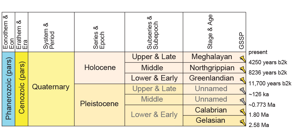
Geologic eons are broken up into eras and eras into periods. Geologic periods are broken up into epochs and epochs into ages. During the Cenozoic Era, the Paleogene Period is broken up into the Paleocene, Eocene, and Oligocene Epochs. The Neogene Period is broken up into the Miocene and Pliocene Epochs. Each one of these earlier Epochs is marked by important evolutionary and geologic changes that define these bands of time. The final Period of the Cenozoic, the Quaternary, is divided up into two epochs, the Pleistocene Epoch and the Holocene Epoch. These are all lithostratigraphic terms, defined by sedimentary rock layers. In terms of time, or chronostratigraphic nomenclature, the rock layers that define an epoch are referred to as a series.

THE PLEISTOCENE EPOCH

Figure \(\PageIndex{5}\): Icehouse and greenhouse periods as recorded in Antarctic ice cores from the last 800,000 years. Greenhouse periods are yellow, icehouse periods are blue. Note that the highest carbon dioxide concentration recorded during this time is around 280pm, versus today’s 415ppm (Source: CC BY-SA 3.0; By Tomruen – Data from ncdc.noaa.gov, and this looks best: Composite \(\ce{CO2}\) record (0-800 kyr BP), marked up with 230 ppm transition between glacial and interglacial periods, https://commons.wikimedia.org/w/inde...curid=16147504.).

The Pleistocene is an epoch of wicked climatic seesaws. At times, there is a layer of ice a mile thick over southern Canada. At other times, there is nearly nothing of that left. We also tend to define the Pleistocene by its fauna, including mammoths, mastodons, saber-toothed cats, and more. The name Pleistocene comes from the Greek and means “most new,” a term given it by Charles Lyell, back in the 19th century. As mentioned above, the base of the Pleistocene is marked by the start of the Gelasian Age, a time when large ice sheets began to grow in higher latitudes around the world. Based upon there being 40 marine isotope stages identified during this time, there were likely at least 20 glacial cycles during this age. The age ends at 1.8 Ma with the extinction of the nannofossil Discoaster brouweri.

Figure \(\PageIndex{6}\): The Pleistocene Series of the Quaternary System (Source: ICS).

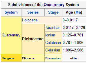
The story of the Pleistocene continues stratigraphically upward into the Calabrian Age (1.8 Ma to 0.774 Ma) into the Chibanian Age (0.774 Ma to 0.129 Ma) and finally to the “Upper” Age (proposed “Tarantian Age,” 0.129 Ma to 0.0117 Ma). The boundary between the Calabrian and Chibanian is marked by the Earth’s last magnetic reversal, but the boundary between the Chibanian and “Upper” Age is marked by the onset of the Eemian interglacial, which is the last warm period before the onset of the Holocene Epoch. Currently the “Upper” Age of the Pleistocene is under consideration for a new name, the Tarantian Age. However, as of just a few years ago from the time of this writing (June 2020), neither a lower or upper GSSP had been defined. In 2018, the upper boundary of a potential Tarantian Age was defined by the onset of the Greenlandian Age of the Holocene Epoch, as defined by a layer within a core taken from the Greenland ice sheet by the Greenland Ice Core Project. The very top of the Tarantian Age occurs at the end of a brief return to icehouse conditions after a significant warm up. This event is referred to as a the “Younger Dryas” and its end is the beginning of the Holocene Epoch and the Greenlandian Age.

This all may seem complicated, full of funny names and obscure dates. There is truth to this on the surface. However, when you peel away all of this complexity, we have described a model that does something conceptually simple: the geologic time scale helps us define time through the environmental change. The model is useful because it is so adaptable.

A Clima(c)tic sidebar – The Younger Dryas

What is the “Younger Dryas,” you might ask? The event itself was a brief return to icehouse conditions at the very end of the Pleistocene Epoch. This kind of funny-sounding name actually references a particular indicator plant, Dryas octopetala, an alpine-tundra wildflower that became more prevalent during this time. We know this because its pollen became more common in lake sediments.

It is called “Younger” because it is the last of three similar sudden cooling phases during a much longer, gradual, warming from the last glacial maximum. The others are called the “Oldest Dryas” and “Older Dryas.” The Younger Dryas begins after a period of gradual warming that had lasted from 24,000 years ago to 12,900 years ago. For about 12,000 years, the Earth had been slowly warming, emerging from a long icehouse period as had been the cycle since the start of the Pleistocene 2.58 million years ago. Then, quite suddenly, actually in the course of just a few decades (a human lifetime or less), the global climate reverted to an icehouse period for another 1,000 years, until 11,700 years ago.

Figure \(\PageIndex{7}\): Temperature proxy record from oxygen isotopes for the period surrounding the Younger Dryas event. Note the rapid warming that occurs at the end of the Younger Dryas. This rapid warming, during most interstadial periods, is followed by several hundred years of gradual cooling. This has not been the record of the Holocene Epoch (Source: By Daniel E. Platt et al., https://commons.wikimedia.org/w/inde...curid=79219152).

What caused this particular climatic event is complicated and not fully understood. It is particularly interesting because of the rapidity of the cooling, which has its counterpart in today’s similarly rapid warming at the hand of humans. Humans, however, did not cause the rapid cooling of the Younger Dryas. But, what did? There are three hypotheses worth exploring. None of them are conclusive, but because the question is open, science is at work.

Hypothesis 1: One hypothesis for the onset of the Younger Dryas is the Vela Supernova explosion that took place at that time. In the constellation Vela, a massive star exploded. Energy from this event is suggested as the cause of the observed evidence for the destruction of the ozone layer, changes in nitrogen levels at Earth’s surface and in the atmosphere, megafauna extinctions, and changes in some stable isotopes. However, there is little understanding of how such events could cause these things. So, while you can read about this hypothesis, there is little support for it.

Hypothesis 2: A second hypothesis suggests that a volcano in southern Germany, Laacher See, erupted. An unusual volcano, a “maar lake,” it is today a low-relief crater about 2km in diameter. It is calculated that the eruption at the time would have been large enough to send enough material into the atmosphere to account for the degree of cooling during this period. However, it has not been studied thoroughly enough.

Hypothesis 3: A third hypothesis proposes a bolide impact large enough to cause the climate change observed. A wide variety of evidence exists from sites around the world for their having been such an impact at that time. These include grains of melt-glass and nanodiamonds. What was missing was a crater of the right age. In 2018, under a glacier called “Hiawatha” in northern Greenland, researchers found a massive crater that may fit the bill. At 31km wide, it is not as large as Chicxulub (the dinosaur extinction crater), but represents the effects of what was likely an iron asteroid 1.5km across slamming into the Earth at the time. Its timing is still up for debate, as it could be as old as 100,000 years or as young as 12,900. More research will bring answers.

Figure \(\PageIndex{8}\): The Holocene Epoch is directly preceded by the Younger Dryas climate event at the end of the Pleistocene Epoch. Whatever caused the Younger Dryas, it was a short-lived cold excursion (Source: Public Domain, https://commons.wikimedia.org/w/inde...curid=73612526; By United States Geological Survey – https://pubs.usgs.gov/pp/p1386a/gallery2-fig35.html).

Figure \(\PageIndex{9}\): 19th century map of the extent of post-glacial Lake Agassiz created by geologist Warren Upham. The actual lake’s boundaries were likely much greater than the area indicated here (Source: Public Domain).

Hypothesis 4: A fourth hypothesis for this abrupt onset of climate change is the emptying of glacial Lake Agassiz in southern Canada into the North Atlantic via the St. Lawrence seaway. Remnants of this post-glacial lake still exist today and include Lake of the Woods, Lake Winnipeg, and Lake Manitoba, among others. Periodically, this lake would be dammed up by ice, allowing fresh meltwater to accumulate over a very large region. There are five identified phases in all in the record. When the glacial dam would burst, massive volumes of freshwater would enter the North Atlantic and disrupt the current thermohaline circulation and significantly alter global climate.

Did I Get It? - Quiz

Exercise \(\PageIndex{1}\)

In chronostratigraphic terms, an Epoch is equivalent to a ___________. Rocks contained in such units can be directly linked to a particular geologic Epoch, independent of geographic location.

a. Series

b. Stage

c. Unit

d. System

Answer

a. Series

THE HOLOCENE EPOCH

Figure \(\PageIndex{10}\): Quaternary System subdivisions, including the Holocene and its newly accepted Ages (Source: ICS).

Holocene, from the Greek, means “Entirely New.” For 11,700 years (since 11.7 ka), the climate on our planet has been remarkably stable. Because of this stability, our own species has been able to not only flourish, but to spread well beyond the geographic ranges and biomes to which it was limited during the Pleistocene. While our hunter-gatherer ancestors within the genus Homo have been wielding fire as far back as 1.2 million years, they relied only on what the land provided them for all of that time when it came to food and shelter. That meant hunting game, gathering fruits and plants, and more. The long stability of Holocene climate, combined with our species’ cultural development up to that point, made technologies leading to agriculture, via the Neolithic Revolution, possible. This revolution would provide new sources of food, through the artificial selection of grains and subsequent plants (and animals, eventually), that no longer required consistent or even just seasonal movement. It was possible to settle in one place, develop towns, eventually cities, and the specialization and division of labor. It may have also made it already possible for our species to alter the planet’s climate. More on that in a moment...

Unusual Stability – Sort Of...

Is the Holocene’s climate unusually stable? When compared to other spans of time between ice ages, including the last interglacial (the Eemian), there are many similarities in terms of temperature and duration. The Holocene Epoch is one of the longest interstadial periods on record. This being said, there are some noteworthy departures from this stability that are worth exploring. As of 2018, two of these have been used to further divide our epoch into ages.

Figure \(\PageIndex{11}\): Oxygen isotope records for five Greenland ice cores. Note the isotope excursions at 8.2 ka, 9.3 ka, and 11.4 ka. Otherwise, the Holocene climate has been very stable (Source: University of Copenhagen Centre for Ice and Climate).

Subdividing the Holocene: Climatic Ages

While there have been one or two attempts in past decades to further subdivide the Holocene Epoch, nothing stuck. The Quaternary, in general, is overwhelmingly defined by ice ages. Because Quaternary stratigraphy is overwhelmingly defined by deep sea marine sediments and ice core markers, it is reasonable then to assume the task of subdividing the Holocene Epoch would be no different.

Figure \(\PageIndex{12}\): Holocene temperature reconstructions taken from 8 published sources (Source: Wikimedia Creative Commons).

However, the Holocene is not punctuated by long-lasting changes in climate. A three-part division was proposed based upon ice core and cave speleothem data. The base of the Holocene Epoch, the Greenlandian Age, and the subsequent Northgrippian Age, have GSSPs marked in ice cores, NGRIP2 and NGRIP 1, respectively. Our current age, the Meghalayan Age, is recorded in a speleothem record from a cave in Meghalaya, India. Within the boundaries of the Holocene Epoch, two major climatic events of note can be picked out during the 11,700 year long Holocene, one at 8.2ka (ka = thousands of years ago, or kiloannum. “ka” and “ky” are historically interchangeable) and the other at 4.2ka.

The 8.2 ka event – The Greenlandian Age ends and the Northgrippian Age begins

The base of the Holocene begins at 11.7ka with the Greenlandian Stage GSSP recorded in the NGRIP2 ice core. But what happened? Why is it noteworthy? It is located at a depth of 1492.45m where a shift to heavier \(\delta\)\(\ce{^{18}O}\) values is recorded. In stable isotope science, we can use the environmental fractionation, or separation, of isotopes of some elements to tell us something about temperature, moisture, or other variables. Because \(\ce{^{16}O}\) and \(\ce{^{18}O}\) move around in the environment in different and predictable ways, we can use this particularly isotopic pair as a paleothermometer. to understand the Greenlandian/Northgrippian transition, oxygen isotope thermometry is a key. Below is an excellent discussion of the basic science of these methods.

Figure \(\PageIndex{13}\): Central Greenland reconstructed temperature from GISP2 data. Note the temperature departure at 8.2ky (Source: CC BY-SA 3.0; By Giorgiogp2 – Own work, https://commons.wikimedia.org/w/inde...curid=13309952).

In the ice, according to Walker, et al. (2018), the change is quite rapid, taking place in just a few years. Accompanying the changes in \(\delta\)\(\ce{^{18}O}\) were similarly abrupt declines in deuterium values, a reduction in dust concentrations, and a reduction in Na (sea salt) values. This evidence denotes a sudden cooling, very likely on a global scale, as recorded in central Greenland ice core reconstructions.

At 8.2ky, the Greenlandian Age ends, giving way to the Northgrippian Age. This GSSP is defined by a boundary in the NGRIP1 Greenland ice core at a depth of 1228.67m. Walker, et al. (2018) describe this interval as representing a clear signal of climate cooling during an otherwise warming interval of the Holocene. Recorded in a wide range of proxy records around the globe, it is significant because it is relatively short-lived.

The cause of this event is not entirely certain, though it is typically attributed to the release of fresh, cold glacial meltwater from Lake Agassiz and Ojibway into the north Atlantic. These proglacial lakes were quite large, located between today’s Lake Superior and the Hudson Bay in southern Canada. They are survived today by a wide variety of landscapes, including Lake Winnipeg, Lake Manitoba, Lake of the Woods, and other bodies of freshwater from northern Minnesota well into the Canadian provinces of Saskatchewan, Manitoba, and Ontario.

Figure \(\PageIndex{14}\): Maximum extent of proglacial Lake Agassiz (Source: University of Manitoba Libraries Map Collection).

Water likely spilled through the Great Lakes and St. Lawrence Seaway in a great rush, released by a glacial dam. This type of event is called an outburst flood. The sudden infusion of so much cold freshwater into the north Atlantic would have upset the thermohaline circulation in the ocean. This circulation moderates northern temperatures and the shutting off of the current would have caused a significant cooling event, particularly in the northern hemisphere, but with global importance. This cooling could have been as rapid as 3.3\(^{\circ}\)C in just 20 years. Spotty records in tropical regions such as Indonesia also bear records that show a similar cooling, indicating that it was not just an Arctic event. Globally, atmospheric carbon dioxide dropped by 25 ppm over the next 300 years.

The 4.2 ka Event

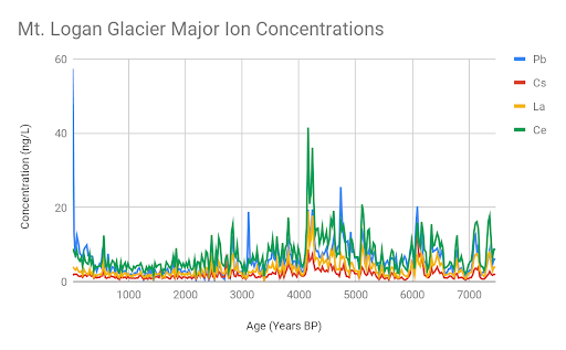
The Northgrippian Age would come to an abrupt end with a another global cooling event, this time accompanied by significant aridification. In 2018, the International Commission on Stratigraphy officially identified the GSSP for the event in a speleothem formation from Mawmluah Cave in Meghalaya, India. As a result, the new age is called the Meghalayan Age. It is the current geologic age in which we live. There is also an auxiliary GSSP contained in an ice core from Mt. Logan, Canada.

Figure \(\PageIndex{15}\): Major ion concentrations from Mt. Logan glacier, the auxiliary GSSP for the Meghalayan Age, Alaska and the Yukon Territory The major ion spikes around 4200ky are consistent with increased airborne particulates due to widespread aridification around the globe.

At the outset of the Meghalayan, many places around the world became much, much drier. This includes large regions of every continent. Changes in east Indian and Chinese monsoons were triggered, moving patterns further to the south than they had before. With changes in weather patterns that would last well over a century, human civilizations at the time were impacted. The degree of this effect is debated among archaeologists and climatologists, but the 4.2ky event coincides with the end of the Old Kingdom in Egypt, the Akkadian Empire in Mesopotamia, the Lianzhu Culture in China, and the Indus River Civilization in India.

Figure \(\PageIndex{16}\): Global distribution of the 4.2ky event, as shown by hatched (wet conditions) and dotted (dry) areas. Source: By Jianjun Wang, Liguang Sun, Liqi Chen, Libin Xu, Yuhong Wang & Xinming Wang – The abrupt climate change near 4,400 yr BP on the cultural transition in Yuchisi, China and its global linkage. (CC BY-SA 4.0.)

Figure \(\PageIndex{17}\): Speleothem from Mawmluah Cave, Megahalaya, northeast India. The position of the 4.2ka event is shown. This specimen is 308mm long. (Source: Walker et al., 2018).

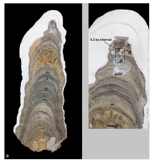
The GSSP itself is marked in the speleothem by a marked reduction in rainfall at 4200 years BP. Evidence from other regions suggests major oceanic and atmospheric changes, particularly in circulation patterns, sometimes referred to as the “Holocene Turnover.” The event appears to have been global. Evidence for this period of aridity is recorded in many locations around the world, including north Africa, the Middle East, and around midcontinental North America. Glaciers record the event in locations like Kilimanjaro, the Andes, and flowstone in Italy. In the northern hemisphere, glaciers re-advanced due to cooling. In mid- to low latitudes, it was marked by aridification in many areas along with disruption of the westerlies, the Indian Summer Monsoon, and the East Asian Summer Monsoon. The resulting megadrought seems to have lasted about 250 years.

Figure \(\PageIndex{18}\): Oxygen isotope record from the speleothem in Mawmluah Cave, Meghalaya, India. The spike that occurs around 4200ky is the GSSP for the Meghalayan Age and marks a severe drying event.

This ends the major official divisions of the Holocene. However, the 8.2ky and 4.2ky events are not the only climate “blips” during the epoch. Two other minor ones occur much later on. Ironically, these have received the most attention over the past few decades, so it is possible you have heard of them.

Did I Get It? - Quiz

Exercise \(\PageIndex{1}\)

Geologic Ages are the shortest lithostratigraphic unit and are equivalent to Chronostratigraphic Stages. The Holocene Epoch now has three Stages. Which of these is not one of them?

a. Greenlandian

b. Northgrippian

c. Meghalayan

d. Calabrian

Answer

d. Calabrian

The Medieval Warm Period

Figure \(\PageIndex{19}\): Hvalsey Church, Greenland, part of a Viking settlement constructed during the Medieval Warm Period (Source: Wikimedia Commons).

The Medieval Warm Period lasted between the years 900 and 1300 CE. It is also sometimes referred to as the Medieval Climate Optimum or Anomaly. For the north Atlantic region, the climate was marginally warmer than the period following up to the mid-20th century. It can be seen in the GISP-2 ice core from Greenland. Possible causes of this anomaly include changes increased solar activity, decreased volcanic activity, or even changes in ocean circulation. There is not strong evidence that it was a global event.

Figure \(\PageIndex{20}\): A reconstruction of what the Viking settlement at L’Anse Aux Meadows, Newfoundland, Canada, may have been like. (CC BY 2.0; Photo by Dylan Kereluk.)

In western culture, the focus on this period is largely due not only to the cultural effects it had on mainland Europe, but as a cause for trans-Atlantic exploration, particularly by the Norse. During this time, groups of Norse colonized Iceland, then Greenland, and eventually reached North America (Newfoundland’s L’anse Aux Meadows) around 1000AD under Leif Erickson. Beginning around 985 CE, Greenland became an important settlement, getting large and stable enough for the Catholic Church to send a Bishop. Walrus tusk, collected for its ivory, was a major export.

Even during this time, however, the Greenland climate was quite harsh, requiring that cattle be contained within stone and earthen barns with walls 10 feet thick for nearly eight months of the year.

Figure \(\PageIndex{21}\): Data showing 11 different published reconstructions of temperature during the last 2000 years globally. Redder colors are more recent reconstructions, bluer are older. Black shows instrumental record data. (Source: CCAS 3.0 Unported; Global Warming Art)

The Little Ice Age

Eventually, it became much harder to make a living in Greenland. This was not just due to economics, but also to the onset of the Little Ice Age. As shown in the temperature reconstructions above, this period of cooling occurred directly after the Medieval Warm Period. Again, it was not necessarily global and may have been a regional event in the north Atlantic. It lasted from about 1300 to 1850 CE, the traditional start of the industrial revolution in Britain.

Possible causes have been proposed include the usual suspects: changes in solar radiation, increased volcanic activity, and changes in ocean circulation, among others. Even decreases in human population has been proposed as a cause, due to the Black Death plague that killed millions of Europeans during the 14^th century. In any case, life in Europe during this time was a mix of hardship, cultural Renaissance, and exploration. The latter was largely motivated as a search for resources to supply a now very resource-poor continent. The cultural and climatic ramifications of this exploration echo into the present day.