12.5: Pattern Matching and Stratigraphic Correlation

Millions of years of weathering and erosion shape our landscapes. Over that time, the records of deposition in ancient basins are washed away, often leaving only sparse remnants of these strata. Measured stratigraphic sections, separated by great distances due to erosion, provide the record necessary to reconstruct these larger ancient environments. The process of connecting layers across these distances is called correlation. Such correlation typically focuses on thicker strata, but can also be done in some cases with microstratigraphic strata, such as minute beds of fossils, volcanic ash beds, impact deposits, etc. Stratigraphic correlation is about making connections. It is a set of scientific activities that seek to match rock patterns across distances.

There are a wide variety of ways that stratigraphic patterns are identified and matched, and quite commonly, the patterns do not match up perfectly. Bedding thickness varies over distances. Beds “pinch out” between outcrops. Sometimes, in some places, a new bed is introduced. Physical or chemical characteristics may be missing. The reasons for these variations are multiple. Simple way to consider these variations is to imagine walking along the coast of eastern North America, and observing the changes you see. While there are many commonalities between the beaches of Florida, Virginia, and New Jersey, changes in the shape of the shoreline, development of large bays, variations in water chemistry, the presence or absence of barrier islands, subtle climate variations, inflowing river channels, the slope of the continental shelf, and a great many other features along a coast will cause shoreline conditions to change. As a result of these natural physical variations, populations of organisms and even entire ecosystems will vary, too. Post-lithification processes can also erase physical and chemical characteristics of the rocks through compaction and diagenesis. All of this natural variation can make correlation quite tricky! Stratigraphers, the geoscientists who study patterns within sedimentary rock layers, have developed a variety of complementary methods that aid in correlation between sites. Ultimately, these tools help establish relative age connections between distant units sometimes separated by millions of years of erosion, tectonic uplift and change, and other geological processes.

Dual GigaPans of Tonoloway Formation along Corridor H. You are seeing two sides of the highway at the same location. Click on the title of the Gigapan and then make it full screen so that you can play with the images. How would you go about correlating these layers from one side to the other? For what distinctive features might you look? List some in the quiz below.

Dueling Tonoloway Outcrops - Quiz

Exercise \(\PageIndex{1}\)

Identify a feature contained within each of these outcrops that you could use to correlate across the road at this location. They are the same rock layers, separated by well over 100 ft of road (Corridor H, West Virginia, Tonoloway Formation).

a. Tracing out a distinctive bed.

b. Road Signs

c. Vegetation

d. Composition of the talus (loose material at the base of the outcrop)

Answer

a. Tracing out a distinctive bed.

Patterns that emerge from measured stratigraphic sections represent not only environmental changes on various scales, but also record the local interactions with the biosphere, atmosphere, hydrosphere, and even with the exosphere, the space environment. If stratigraphy is a record of events in a basin over time, then it will be recorded in complex ways due to these interactions between systems. There will be a record of climate change and large-scale weather events, biosphere events, evolutionary change, changes in the Earth’s magnetic field, and astronomical events that leave an impact (pun intended!). Such changes will often be global and regional in nature and occur across different environments, requiring an analysis focused on events in time across a region. Over the years, stratigraphers have developed various subfields to help provide focused study in these areas. These subfields of stratigraphy include chronostratigraphy, lithostratigraphy, biostratigraphy, and magnetostratigraphy. Together, these fields provide tools that allow the piecing together of the geological past.

Lithostratigraphy

The name, lithostratigraphy, comes from the Greek words lithos, meaning rock, and strata, meaning layers. So lithostratigraphy is the study of rock layers. In lithostratigraphy, we are very interested in the sediment grains that make up these layers. We want to know their mineral composition. We want to examine their shape, whether they are rounded or not. We also want to know something about their sorting, whether they contain a diverse mix of grain sizes or just one grain size. These pieces of evidence describe, in part, the “facies” of the rock,which allows scientists to determine how the rock was formed and where it might have originated. In a stratigraphic section, stacked strata will often come vary from bottom to top, indicating a detailed record of environmental change. This record provides a history of the sediment deposition in that basin, changes in sea level, and can also provide important insights into climate fluctuations, all at a variety of time scales.

In lithostratigraphy, rock strata are placed in a hierarchy based upon several factors. Key among these is their lateral regional extent. The basic lithostratigraphic unit is called the formation. In order to be given this designation, a layer of rock must be mappable across an area. It must bear the very similar characteristics when seen in locations across that area,and have similar, distinct boundaries, or contacts, with layers above and below. Formations are the units used by field geologists when creating geologic maps. Formations also have a “type section” identified that represents the outcrop for which the standard description of the unit was created. They also have contacts with formations above and below, which are also mappable. Within formations, samller subunits called members can be identified. A member is a lithologically distinct bed within the larger formation. In stratigraphic columns below, the Kope Formation is divided into several members. And, within these members, beds are often discernable. The type Cincinnatian is an ideal section for the study of individual beds, as they are often laterally extensive and therefore traceable across the region. A single limestone bed, such as those numbered as 25-31 in column C below, mark distinct moments in time across the region. If enough stratigraphic sections exist from across a region, further patterns will emerge. Roadcuts, cliff faces, and other locations are ideal study areas. Individual rock layers may or may not be present in all of these. They may vary in thickness and content. But this information can help reconstruct the history of not just a single location, as represented by one section, but an entire region.

Figure \(\PageIndex{1}\): Upper Ordovician stratigraphy of the Cincinnati, Ohio region. A) Generalized stratigraphy of uppermost Mohawkian and lower Cincinnatian Series. BR Bromley Shale; LSS lower strophic Sowerbyella rugosa interval; MK Mohawkian Series; PP Point Pleasant Formation; SH Shermanian Stage. B) Stratigraphy of middle and upper Kope and lower Fairview Formations, showing Kope submembers . C) Detailed stratigraphy of the Alexandria submember and the upper Snag Creek (SC) and lower Grandview (GV) submembers. Numbers immediately to left of column are meter-scale cycle designations; numbers to right are designations of cycle-bounding limestone beds (Adapted and used with permission: Kirchner and Brett, 2008).

Normal Fault in Chalk – Correlation of both sides of the fault. Try to match the two sides up be moving the gigapan images around. Can you get ride of one of the faults? If so, you just correlated layers!

Lithostratigraphic Hierarchy

Flow (if volcanic materials are included) \(\rightarrow\) Bed \(\rightarrow\) Member \(\rightarrow\) Formation (Basic Lithostratigraphic Unit) \(\rightarrow\) Group \(\rightarrow\) Supergroup

Packages of formations can be put together into groups. Packages of groups can be assembled into supergroups. Such higher designations are not always necessary or ideal, but in situations where the rock formations are closely related, their use makes good sense. The Grand Canyon Supergroup and the Belt Supergroup are two well known American examples of this largest designation.

Fossils as Stratigraphic Tools: Biostratigraphy

Figure \(\PageIndex{2}\): A simple example of biostratigraphic correlation (CC BY-SA 3.0; By דקי – אני יצרתי, https://commons.wikimedia.org/w/index.php?curid=17935309)

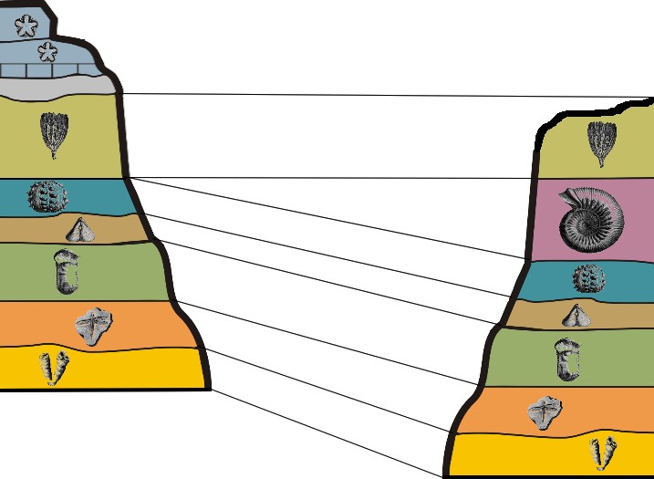
Biostratigraphy is a set of tools used to correlate patterns and beds using fossils. Fossils come in a variety of forms, either as body fossils, such as skeletal parts or impressions, or trace fossils, evidence of movement or activity. Usually, this information is collected in addition to the lithostratigraphic information. Biostratigraphic designations are based upon the existence of a particular diagnostic feature within strata specific to fossil material. Sometimes, such fossil material can be traced over great distances, much like lithostratigraphic layers (Kohrs and Brett, 2008). Biostratigraphic units can vary across a location and so such tracing of fossil beds is not necessarily a basic goal of biostratigraphy. Communities within an ecosystem vary across an environment, depending upon physical and biological conditions. Water depth, temperature, salinity and currents, along with sedimentation rates and nutrient levels can cause the distribution of particular organisms to be quite spotty. However, some fossils are more ubiquitous, for instance due to planktonic life habits, and so are found more commonly over larger areas as they are spread by currents. Because of all of this variation, while biostratigraphic designations can be used to correlate beds, they are also very important tools for understanding the paleoecological history of a location.

Index Fossils

Figure \(\PageIndex{3}\): Some common index fossils (Source: USGS)

Across basins or even within a basin, fossil assemblages can vary a great deal. Consider a modern oceanic shoreline, even one with a barrier island system like the Outer Banks of North Carolina. In such areas, there are species that live across facies, and species whose lives are spent entirely within more restricted zones. Species with a broader distribution, that are plentiful, and that fossilize well can serve very well as markers for important intervals. Ideally, the organism’s existence is short-lived. If all of these criteria are met, then that fossil can serve as a marker in strata, an index fossil. Some excellent examples of index fossils can be found here.

Biozones

Biostratigraphy comes with its own unique set of terminology. Unlike chronostratigraphy and lithostratigraphy, there is no hierarchical system of designations. The biozone is the basic element. Biozones are defined by the basic characteristics of their fossil taxa. There are five kinds of biozones. These include range zones, interval zones, assemblage zones, abundance zones, and lineage zones. Due to the lack of hierarchy, and the variety of ways biostratigraphic designations can be made (by single fossils or multiple fossils present), it is possible to have overlapping biozones within a single rock unit.

Figure \(\PageIndex{4}\): Fossil occurrences, stratigraphically, within the Alexandria Submember of the Kope Formation. This data was compiled from studies at six sites. Fossil occurrences at 5-6 sites are indicated with black bars. Gray bars identify fossils found at 3-4 sites. Light gray bars indicate fossils found at 1-2 sites. Dark gray to black bars could be considered fossils zones (range zones) useful for biostratigraphic correlation (Kohrs, 2003).

Range zones come in two varieties. The first, a taxon-range zone, is defined as a body of strata with a geographically and temporally defined occurrence of a single fossil taxon. The geographic range can be narrow or very broad, but is defined by the entire known set of occurrences of that taxon across the basin or set of basins where it has been identified. The second, concurrent-range zones, are only different from the taxon-range zone in that they consist of overlapping ranges of at least two taxa. Range zones can be used for stratigraphic correlation across locations, due to their geographic extent.

Interval zones are the fossiliferous strata that exist between two defined stratigraphic horizons. These are sometimes referred to as range zones. For instance, you will not find fossils of modern humans going back more than at most 350,000 years. The interval zone of our species only represents the last 350,000 years. Interval zones are bounded by the occurrence of the taxon in question, so do not necessarily have a correlative power. However, because they are defined by lower and upper horizons, these horizons can be used as stratigraphic correlation markers.

Lineage zones are defined by their evolutionary importance. They are zones that contain a particular evolutionary branch of a taxon. These very specific biohorizons, again defined by their lower and upper limits of occurrence, are very reliable means of relative time correlation in biostratigraphy. It is one thing to be able to correlate across a region the existence of a particular family or genus of a brachiopod, but quite another to be able to define a correlatable time horizon using a specific species.

Assemblage zones are defined by the lower and upper boundaries of strata that are defined by the presence of three or more fossil taxa. These taxa may represent members of a community within the paleoenvironment defined by the strata in which they are contained. Across a region, not all members of the assemblage need be present to be defined in this way, but most of them should. Individual taxa can also have more extended ranges above and below the assemblage zone.

Abundance zones represent a body of strata where the abundance of a particular taxa is significantly greater than usual. The Triarthrus eatoni zones in the figure below from Kohrs (2008) can be defined as abundance zones within the context of a single location, though such zones are potentially also correlative tools. This trilobite can be found here and there within the Kope Formation, but at each one of these localities, could be found in unusual abundance and preservation as a fossil lagerstätte. As correlative markers, they mark a particular useful biohorizon.

Figure \(\PageIndex{5}\): A lithostratigraphic and biostratigraphic interpretation of mudstone (gray) and limestone (white) layers within the Alexandria Submember of the Kope Formation in the Cincinnati/northern Kentucky region. Each column represents a different location across a transect covering over 50 miles of distance. These columns all represent sediments deposited in the same basin and during the same interval of time. Limestones and fossils can be correlated, or matched by patterns, across the region (Kohrs and Brett, 2008).

Abundance Zones or Lack Thereof: Fossil Lagerstätten, Epiboles, and Outages

Figure \(\PageIndex{6}\): An exquisite speciment of Cryptolithus bellulus from the Alexandria Submember of the Kope Formation, Cincinnati, OH (Kohrs and Brett, 2008).

Some fossils are exceptional in how they are preserved. Exceptionally rich fossil deposits are given the name lagerstätten, a German term that literally means “storage place” because the preservation is so exquisite as to represent what the original organism was like in appearance. Such fossils can sometimes be found in beds that are traceable as units across a region, their exception preservation being caused by the rapid deposition of sediment downslope during a storm event or by some other means. As such, they can be used as important biostratigraphic marker beds (Brett and Baird, 1997).

Figure \(\PageIndex{7}\): Fossil specimens, molts of the trilobite Triarthrus eatoni, from the Alexandria Submember of the Kope Formation, Cincinnati, OH. An exquisite fossil lagerstatten, these particular specimens could be indicating behavior. As these are molts, there are one of two options for how they arrived to be buried here. A large concentration of these molts managed to concentrate here from further upshore. Or, these molts indicate potential mating behavior, as the arthropod shed its exoskeleton (Kohrs and Brett, 2008).

In general, beds that are stratigraphically traceable across a region may contain fossils that appear in one place but not in another. Fossils are suddenly very abundant in bed or formation may represent what is referred to as an epibole, or a sudden flourishing of a species or community in the stratigraphic record. These can at times be important event beds for correlation across a region. Likewise, the opposite of this is an outage, which represents the disappearance of a fossil or community. This could even be a localized extinction event (e.g., Brett and Baird, 1997). Again, such outages can be important biostratigraphic event be markers.

Principle of Faunal Succession

Because of the way evolution has influenced life on Earth, there is a distinct sequence of appearances of organisms through time. This sequence of life begins four billion years ago, with the appearance of single-celled prokaryotic microbes. Since then, origination and extinction have formed and killed off numerous species, always giving way to new species with novel adaptations based upon shared and derived characteristics. Important patterns develop across the fossil record that allow paleontologists to identify rock units as being of a certain age or environment. It is known, for instance, that humans never lived with dinosaurs. Human fossils have never been found with, among, or in units with dinosaur fossils, and these groups of fossils are separated by at least 61 million years of time, sediment, and events. If a rock contains a dinosaur fossil, we can thus tell that it is at least 65 million years old but not more than 243 Ma (Nyasasaurus parringtoni). If it contains a human fossil, our species specifically, it is likely less than 500,000 years old.

Chronostratigraphy

Some sediments are deposited at the same time within a basin, but within different depositional environments. Likewise, at any given point in geologic time, multiple basins around the planet accumulate sediments depending on regional tectonic and climatic conditions. Chronostratigraphy, or stratigraphy based upon time, provides a way to correlate units that would otherwise seem to be unrelated. Chronostratigraphy uses aspects of biostratigraphy and numerical dating to constrain the time of deposition within basins using notable fossil beds and other unique features, like volcanic ash deposits.

Chronostratigraphy places strata in a hierarchy based upon radiometric dates calculated from sampling minerals in a rock, rather than relying solely on physical features in the rock. Common examples of such markers are volcanic ash layers, magmatic intrusions, and zircon crystal inclusions. Globally, the International Commission on Stratigraphy (ICS) has created a time chart based upon an agreed global chronostratigraphy. Each boundary on this time chart is marked by a GSSP, or Global Stratotype Section and Point. A GSSP is a chronostratigraphic “type locality” where that boundary has been marked as the example for entire geological community. Global chronostratigraphic names can be different than regional names for these periods of time. There is a long tradition of applying regional names to rock and time units in the geosciences. Many of the names on the geologic time scale, such as Cambrian and Devonian are derived from locations in Europe. Sometimes, old regional names fall away in favor of others. Among scientists, more regionalized names become a part of the common geological vernacular, where there may be much less familiarity with global designations. For example, the Cincinnatian Series is the local name in the eastern United States for the global Upper Ordovician Series.

Chronostratigraphic designations are roughly equivalent to their lithological counterparts. What follows is a table showing the various lithologic units with their chronostratigraphic equivalents.

Comparison of Chronostratigraphic and Lithostratigraphic Designations

How to Name Our Moment in Geologic Time: Lithostratigraphically and Chronostratigraphically	Lithostratigraphic Designation	Chronostratigraphic Designation
Phanerozoic	Phanerozoic Eon	Phanerozoic Eonothem
Cenozoic	Cenozoic Era	Cenozoic Erathem
Neogene	Neogene Period	Neogene System
Holocene	Holocene Epoch	Holocene Series
Meghalayan	Meghalayan Age	Meghalayan Stage

In lithostratigraphy, we refer to stratigraphic units as being deposited within a particular Eon, Era, Period, Epoch, or Age. Associated names, like "Pennsylvanian", can be very regional. In Chronostratigraphy, these basic units have similar names, such as Eonothem, Erathem, etc. However, the names given that accompany these designations are agreed upon global time horizons.

Chronostratigraphic designations and boundaries are marked with radiometric dates. For the GSSPs that do exist, the dates are accompanied by a feature in the rock, such as a fossil zone, magnetic horizon, or other distinctive feature found widely at that time. This combination of factors can be hard to find. Because of this, not all boundaries on the ICS timescale have agreed upon GSSPs. Sometimes, the term “Golden Spike” is used to refer to GSSPs.

“Golden Spikes”

On May 10th, 1869, politician Leland Stanford drove a 17.7 karat copper-alloyed “golden spike” into a wooden railroad tie at Promontory Summit, Utah. At this location, the Union Pacific and Central Pacific railroad lines connected their respective ends of the transcontinental railroad, ending many years of labor and connecting a nation just beginning the long recovery from a civil war. The term “golden spikes” is now used to mark moments of geological importance where significant changes, or shifts, occurred.

Geologically, a “golden spike” is used to mark a boundary on the geologic time scale (note the “golden spikes” on the ICS timetable linked above). “Golden Spike” is a colloquial term used for the more technical Global Boundary Stratotype Section and Point, or GSSPs, that are used to define most boundaries on the geologic time scale. There are rules for marking these, and they are as follows:

• A GSSP has to define the lower boundary of a geologic stage (body of rock deposited during an Age).
  The lower boundary has to be defined using a primary marker (usually first appearance datum of a fossil species).
• There should also be secondary markers (other fossils, chemical isotope signatures, geomagnetic reversal).
• The horizon in which the marker appears should have minerals that can be radiometrically dated.
• The marker has to have regional and global correlation in outcrops of the same age
• The marker should be independent of facies.
• The outcrop has to have an adequate thickness
• Sedimentation has to be continuous without any changes in facies
• The outcrop should be unaffected by tectonic and sedimentary movements, and metamorphism
• The outcrop has to be accessible to research and free to access. This includes that the outcrop has to be located where it can be visited quickly (International airport and good roads), has to be kept in good condition (Ideally a national reserve), in accessible terrain, extensive enough to allow repeated sampling and open to researchers of all nationalities.

GSSP markers provide geoscientists with a common language globally. They also provide common markers that are used to mark boundaries on the geologic time scale. In science, it is important to have a common language that everyone can use for efficient and clear communication. In the story of the rock record, it is important to identify important highlights. While the determination and description of a GSSP is not a flashy act, these markers are used throughout the discipline in a variety of important ways. “End-Permian” is used to discuss a very large mass extinction. “Frasnian-Fammenian”, two stages at the end of the Devonian, is used to discuss that extinction.

Magnetostratigraphy

Like other stratigraphic tools, magnetostratigraphy relies on special properties in the rocks to correlate them across distances. In the case of magnetostratigraphy, the record examined is the recorded inclination and declination of the Earth’s magnetic field at the time of deposition, also known as normal and reverse polarity. This includes correlating times of magnetic reversal, or times when the Earth’s magnetic poles have reversed polarity, with “Geographic South” becoming “Magnetic North”, and vice versa. Operating irrespective of the lithology or fossil content, magnetostratigraphy relies on minerals in the sediment at the time of deposition or in volcanic ash deposited during eruptions, allowing a different set of correlations to be applied.

Magnetostratigraphic “zones”, or magnetozones, are portions of the stratigraphic section that share polarity from the same time period and, within these zones, “magnetic chrons” can sometimes be identified that allow numerical dating of specific moments within such zones. Such zones and chrons, when traceable over distances, contribute unique information about a time period in that location and region, but also complement the tools offered by chronostratigraphy, lithostratigraphy, and biostratigraphy in characterizing the rock record or by filling in knowledge gaps left by them.

Many important GSSPs are marked by magnetozone boundaries. All of the important ratified GSSP boundary markers for the Pleistocene Series of the Quaternary System (1.8ma and 2.58ma) and the Pliocene Series of the Neogene System (3.6 Ma and 5.33 Ma) are marked by magnetic polarity changes in the stratigraphic record. These boundaries mark global changes in the Earth’s magnetic field polarity as seen in iron-bearing minerals. For example, the GSSP for the Gelasian Stage of the Pleistocene marks the end of the Pliocene and the start of the Pleistocene System. This magnetic boundary is described at an outcrop in Calabria, Italy, located just off of the main road near an old farm. In this bucolic setting and contained within the limey muds of the unit, lies a magnetic anomaly that marks an important reversal of the Earth’s magnetic field. You could sample this rock and never see it, as such a boundary is not visible to the eye, but only through a magnetometer. Still, this reversal should be recorded globally and represents an important boundary between two stratigraphic units.