1.1: Introduction

Hopefully you have taken this course because you already have an idea of what remote sensing is, and you want to learn more about it. But what exactly is remote sensing?!?

What is remote sensing?

Some very broad definitions go something like ‘remote sensing is studying something without touching it’. While true in the most basic sense of the words, such definitions aren’t really very useful. Without going into philosophical discussions about what ‘studying’ and ‘touching’ mean anyways, I think we can agree that you are not doing remote sensing right now as you are reading this document on a computer screen… despite learning what this document says without touching it. More appropriately for this course, we can define remote sensing as using an instrument (the sensor) to collect information about the Earth’s surface (or other parts of the Earth, its oceans or atmosphere, or other planets for that matter) at large extents and at some distance. Typical examples include use of satellite imagery or aerial photography, but acoustic sensing (e.g. of the seafloor) and other technologies that do not create data in the form of an ‘image’ are also part of the broad subject of remote sensing. This kind of definition means that another term, ‘Earth Observation’, is often used interchangeably with ‘remote sensing’.

Review of remote sensing technologies

Passive sensing

There are many ways to split existing remote sensing technologies up into categories. Some technologies rely on ambient energy (e.g. energy that is naturally present in the environment, such as sunlight). These are called passive sensing technologies.

Active sensing

Others provide their own source of energy, emitting an energy pulse toward a target area and recording the part of it that is reflected back to the sensor (think about the sonar used on submarines). These are called active sensing technologies.

Optical sensing

Another way to categorize remote sensing technologies is by the kind of energy they use. Some technologies rely on visible light (e.g. traditional aerial photography), while other technologies expand the range of wavelengths sensed to the ultraviolet and infrared (which is also the kind of ‘light’ your TV’s remote control uses). When measuring reflected sunlight in these wavelengths, these are called passive opticalsensing technologies – optical because the instruments employ classic optics in their design. The satellite images seen on Google Earth, or used as a background on televised weather forecasts, are images created with passive optical remote sensing. A form of activeoptical sensing is called lidar, light detection and ranging. It involves emitting a laser pulse (the active part) toward a target and measuring the time it takes before that pulse has hit something and part of it returns to be measured at the sensor. The intensity of the return pulse is typically also measured.

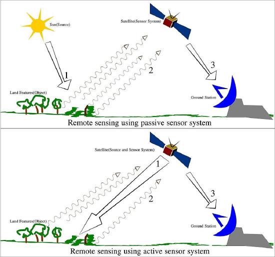
1: The difference between passive and active remote sensing systems. Source: Remote Sensing Illustration by Arkarjun, Wikimedia Commons, CC BY-SA 3.0.

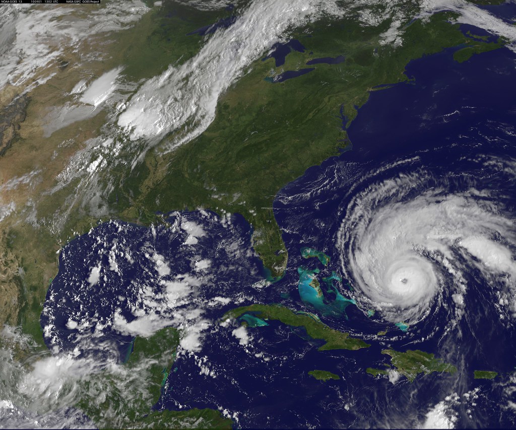
2: NASA Satellite Captures Hurricane Earl on September 1, 2010 by NASA Goddard Photo and Video, Flickr, CC BY 2.0.

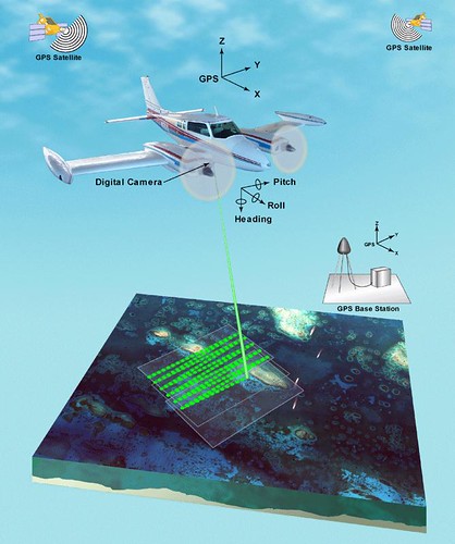
3: Concept diagram for airborne lidar. The location and orientation of the instrument is provided by the GPS and IMU instruments on the aircraft. With this knowledge, distances measured between the instrument and objects on the ground can be converted to find the locations of those objects, together providing a 3D image of the Earth’s surface. fis01335 by NOAA Photo Library, Flickr, CC BY 2.0.

Thermal sensing

Thermal sensing is similar to passive optical sensing except the energy measured by the sensor is in the ‘thermal region’ of the wavelength spectrum. This is the kind of passive thermal sensing you do yourself when putting your hands close to the campfire to feel its heat, so we can feel thermal radiation but we can’t see it with our eyes like we can see sunlight. The Sun produces much more thermal radiation than the Earth does (it is much hotter, after all), but the Sun is also very far away, so if you build a thermal sensor and put it in an airplane or on a satellite and point it towards Earth, the thermal radiation emitted by the Earth overwhelms the small amounts of thermal radiation that has reached Earth from the Sun and been reflected by the Earth’s surface into the sensor. As a result, thermal remote sensing is useful for measuring the temperature of the Earth’s surface.

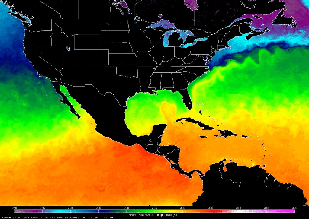
4: This map shows the distribution of Sea Surface Temperature for one day in 2010. Sea Surface Temperature is routinely measured by several satellites, including MODIS Terra that produced the data shown here. Sea Surface Temperature Map (NASA, SPoRT, 04/23/10) by NASA’s Marshall Space Flight Center, Flickr, CC BY-NC 2.0.

Microwave sensing

Moving into the kinds of radiation we can neither see nor feel ourselves, microwave sensing is an important part of remote sensing. The Earth constantly emits small amounts of microwave radiation, and passive microwave sensing can be useful in a way somewhat analogous to thermal remote sensing, to measure characteristics about the Earth’s surface (e.g. where there is snow and ice). Active microwave remote sensing, also called radar remote sensing, uses emitted radar pulses just like radars on ships and at airports. Radars are mounted on aircraft or satellites and pointed toward Earth, radar pulses are emitted, and the reflected part of each pulse measured to provide information about aspects of the Earth’s surface, most of which cannot be measured with optical or thermal technologies. These include information on the Earth’s terrain (for making digital elevation models), soil moisture, vegetation density and structure, and the presence of sea ice and ships. Radar remote sensing has the advantage that microwave radiation moves through the atmosphere more or less unimpeded, and because it is an active technology it can thus be used anywhere at any time, including during the night and in bad weather.

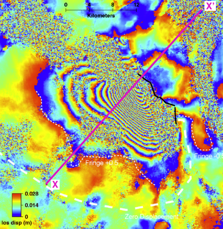
5: An amazing application of radar remote sensing is a technique called interferometric synthetic aperture radar, or InSAR. When a radar instrument passes the same area during two different orbits, changes in the shape of the Earth’s surface can be mapped with millimeter precision. For example, when earthquakes happen the change in the Earth’s surface can be mapped, as shown here for the 2010 earthquake in Dinar, Turkey. Smaller changes that result from e.g. buildings sinking into the substrate or bridges expanding and contracting in hot and cold weather, can also be mapped with InSAR. Interferogram of the Dinar, Turkey 1995 earthquake by Gareth Funning, GEodesy Tools for Societal Issues (GETSI), CC BY-NC-SA 3.0.

Gravimetric sensing

Another kind of instrument that has been put on satellites with great success measured the Earth’s gravity field and how it changes spatially. The Earth’s gravitational pull as sensed by an orbiting satellite is stronger when the satellite passes over an area with relatively large mass (e.g. the Himalayas), as opposed to an area with less mass (e.g. deep oceans). These differences can be measured very accurately and used to not only map the general shape of the Earth’s gravity field, but also to measure changes in it through time. Such changes are caused by tides (more water equals more mass equals more gravity), melting glaciers, and even lowered groundwater tables from unsustainable use of groundwater.

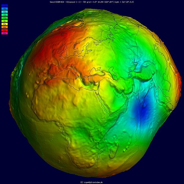
6: Earth shaped and coloured according to gravitational pull as measured by the European Space Agency’s GOCE satellite. Geoid undulation 10k scale by the International Centre for Global Earth Models, Wikimedia Commons, CC BY 4.0.

Acoustic sensing

Acoustic sensing is fundamentally different from the previously listed technologies because it uses acoustic waves (i.e. waves that form as a result of compression and expansion of water masses) while all the others use electromagnetic radiation (i.e. waves that have a magnetic and electric component and can propagate through empty space). While there are many uses of acoustic sensing, primarily mapping water depth, seafloor and even sub-seafloor structure, the instruments and its physical basis are sufficiently different from the previously listed technologies that we will not look at them further in this course.

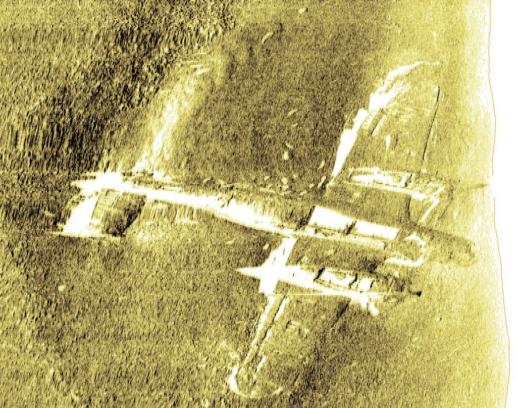
7: Acoustic sensors can both provide information on water depth and substrate composition over large areas, and provide detailed information on seafloor structure in smaller targeted areas. Seen here is a 3D reconstruction, based on acoustic data, of a World War II aircraft located off the UK coast. Aircraft on the seabed by Wessex Archaeology, Flickr, CC BY-NC-SA 2.0.

Land-based sensors

All remote sensing technologies are initially developed and tested in labs on land, where the fundamental science is done, prototypes are produced and tested, initial data are analyzed, and the technology is matured. While some are eventually reconstructed for use in an aircraft or on a satellite, these technologies typically retain their use on land. Well-known examples include the cameras that are in smartphones, the thermal cameras electrical inspectors use to look for faulty circuits, the radars police use to check how fast you are driving, and the lidars some self-driving cars use for situational awareness. While land-based sensors are useful for collection of very precise information from a small area or object, they are not useful for obtaining the kinds of data needed for mapping. Nevertheless, the data produced by land-based instrument are often useful in the remote sensing process (e.g. by comparing what you see in a satellite image to what you measured on the ground).

Airborne sensors

Eventually, someone will take a land-based technology and wonder ‘what would happen if I took that instrument, put it in an aircraft, pointed it down, and turned it on?’. The advent of aerial photography followed quickly after the development of the camera when someone decided to bring a camera up into a hot-air balloon, and airborne lidar and radar systems also followed the development of their respective technologies without much delay. There are at least two challenges that must be overcome when taking a remote sensing instrument airborne. 1) The instrument must be able to collect lots of data quickly, and store this data for later use (or transmit it directly to a storage device elsewhere), and 2) each collected data point must typically be georeferenced – in other words a geographic coordinate pair (e.g. latitude and longitude) must be associated with each data point. These are by no means insurmountable challenges today, when a typical smartphone can act as both data storage and GPS, and putting sensors on airborne platforms has recently become an area in explosive growth because cheap and easy-to-fly drones can now replace manned aircraft as the platform that carries the instrument.

Space-borne sensors

After an instrument has been proven useful when mounted on an aircraft, eventually someone will suggest that ‘we should totally take this and put it on a satellite, so we can collect data continuously for years without having to land, refuel, submit flight plans and so on’. In fact, (to my knowledge) all Earth-observing satellites carry instruments whose prototypes were tested on aircraft, because not only does this help fine-tune the instrument hardware before launching it into space, it also gives remote sensing scientists a preview of what the data from the instrument will be like, so they can start writing programs that process the instrument data and convert it into useful information about the Earth. There are important advantages and disadvantages to the use of satellites compared to drones and manned aircraft. The great advantage is that satellites typically last for many years and can collect data continuously over that period. They are thus incredibly cost-effective. Just imagine what it would cost to provide daily updated information on sea ice cover in the Arctic (and Antarctic for that matter) without satellites! However, satellites have limited fuel, and space is a rough environment so the instruments on board degrade with time and may ultimately fail entirely. For example, in 2012 the multi-billion-dollar European satellite ENVISAT stopped communicating with its command centre, and despite the best efforts by the European Space Agency to resume communication the satellite with all its instruments was declared ‘dead’ two weeks later. Landsat 6, a general-purpose American land observation satellite failed to reach its orbit after launch, and never produced any data at all. One important problem with satellites is that when these things happen, they can’t land and be fixed, as could be done if a problem developed with an instrument sitting in an aircraft.

While the large majority of space-based sensors are located on satellites, other spacecraft have also carried a few important remote sensing instruments. A radar system was placed on a Space Shuttle in 2000 and used to produce a near-global digital elevation model at 30-meter spatial resolution during its 11 days of operation. Recently, a Canadian company called UrtheCast operated two passive optical sensors from the International Space Station – one was an ultra-high-definition video camera that produced video at three frames per second with a spatial resolution of 1.1 meters, the other is a more typical imaging instrument that produced colour imagery at 5-meter spatial resolution.

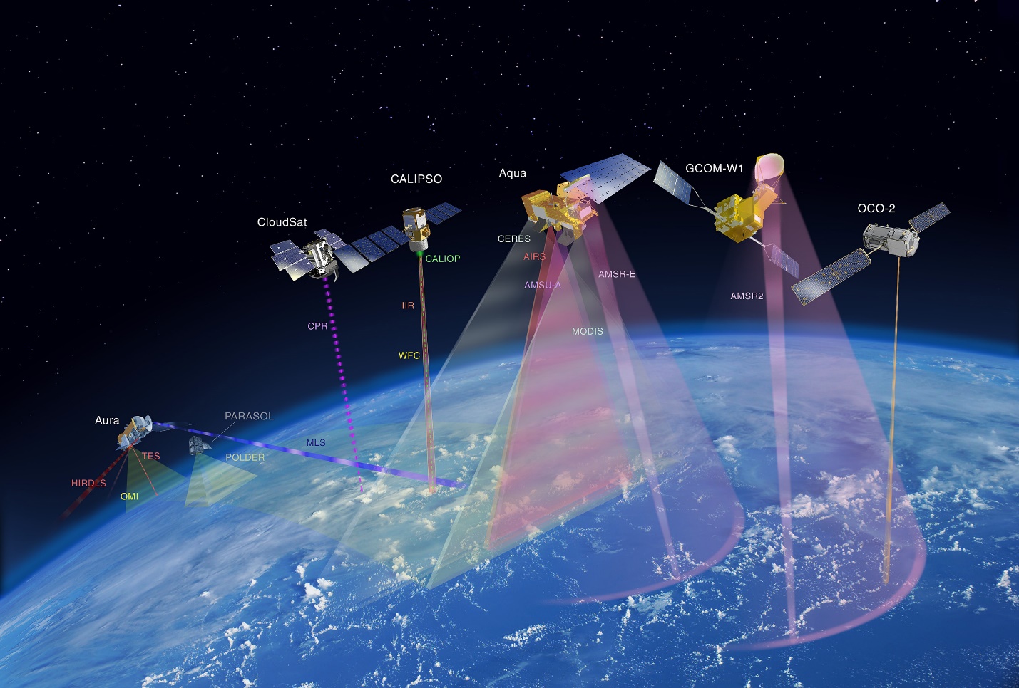
8: There is today a remarkable number of Earth-observing satellites in orbit. This image shows NASA’s ‘A-train’ satellite constellation, a series of satellites whose orbits closely follow each other, all passing overhead during the early afternoon, local solar time. Constellations provide the opportunity to use data from one satellite to aid interpretation of data from another satellite, thus improving the quality of many satellite products. Atrain-879×485 by Shakibul Hasan Win, Wikimedia Commons, CC BY-SA 4.0.

Electromagnetic radiation and its properties

Now it is time to look at bit more closely at how remote sensing works, and what is its physical basis. That will provide you with a better understanding of how remote sensing data are created, and how they may be used in creative ways to extract exactly the kind of information needed for a specific purpose.

The energy that is measured by a remote sensing instrument (other than acoustic instruments), and that is used to produce an image, is called electromagnetic radiation (often abbreviated to EMR). It can be difficult to understand exactly what electromagnetic radiation is, but a useful way to think about it is to consider that light is a specific kind of electromagnetic radiation, one that our eyes and brain are good at detecting. Other kinds of electromagnetic radiation include the harmful ultraviolet (UV) rays that sunscreen provides some protection from, the thermal radiation that we feel when moving close to a campfire, and the radar waves used to detect aircraft and ships (and to map some surface properties on Earth). Physically, electromagnetic radiation can be visualized as waves that propagate through space. The waves have two components, one electrical and one magnetic, which are at 90-degree angles both to each other and to the direction of propagation (Figure 9).

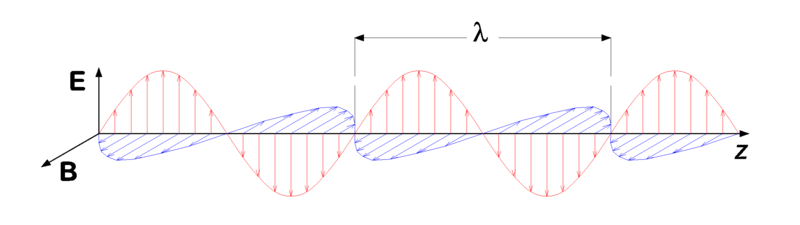
9: Electromagnetic radiation consists of a transverse wave with an electric field (red, vertical plane) and a magnetic field (blue, horizontal plane), propagating (in this figure) in the horizontal direction. Electromagnetic wave by P.wormer, Wikimedia Commons, CC BY-SA 3.0.

Wavelength

EMR waves have certain properties that we can measure and use to describe it. EMR waves can be characterized by their wavelength, which is measured as the physical distance between one wave peak and the next, along the direction of propagation. Human eyes are able to detect electromagnetic radiation with wavelengths roughly in the range between 400 and 700 nanometers (a nanometer is 10-9 meter, or a billionth of a meter), which is therefore what we call visible light. EMR waves propagate at the speed of light, and there is a simple and direct relationship between the wavelength and the frequency of EMR waves, typically expressed as c = νλ, where c is the speed of light, v (the Greek letter nu) is the frequency, and λ (the Greek letter lambda) is the wavelength. The frequency is defined as the number of wave peaks passing a fixed point per unit of time (typically per second). Note that some people, including engineers and physicists working with radiation, sometimes use the wavenumber instead of wavelength or frequency. The wavenumber (ṽ) is defined as ṽ=1/λ. We will not use the wavenumber in the rest of these notes, but it is good to be aware of its use for later studies.

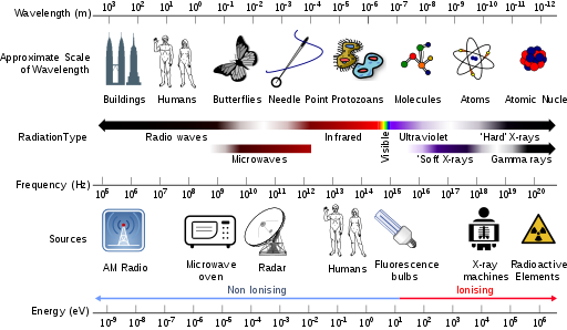
10: An overview of different kinds of EMR, their wavelengths, frequencies, and some common sources. Electromagnetic spectrum with sources by Dinksbumf, Inductiveload and NASA, Wikimedia Commons, CC BY-SA 3.0.

According to quantum theory, EMR can also be considered as consisting of a stream of individual energy packages called photons. Each photon contains an amount of energy that is proportional to its frequency, a relationship expressed as E=hv, where h is Planck’s constant (roughly 6.6 * 10-34 Js). The relationship between wavelength, frequency and energy per photon is shown in Figure 10. Also found in Figure 10 are the common names for EMR of a certain wavelength. You can see, for example, that X-rays have very short wavelengths, very high frequencies, and therefore very high energy content per photon, which is an important reason to limit your exposure to them.

Polarization

In addition to wavelength, EMR can be characterized by its polarization, which can be thought of as the orientation of oscillations of the electric field. For example, in Figure 9, the electric field oscillates exclusively in the vertical plane, so the EMR shown in the figure is said to be vertically polarized. Many sources of EMR, like the Sun, produce electromagnetic waves whose polarization changes so quickly in time that, when measured, the combination of many waves appears to have no distinct polarization. In other words, the orientation of the oscillations of the electric field (and by extension of the magnetic field) is vertical, horizontal, and anything in between. Such EMR is called unpolarized. Other sources of light, such as that created by most instruments, is polarized, meaning that the orientation of the oscillations of the electric field does not change with time. A familiar example of polarization is sunlight reflecting off a water surface. When the Sun’s unpolarized light hits the water surface, the waves whose electric field is oriented vertically are absorbed or refracted into the water more easily than those whose electric field is oriented horizontally, which are more likely to be reflected off the water surface. When you look at a water surface, the horizontally polarized parts of the light you see have thus predominantly been reflected off the water surface, while the vertically polarized parts of the light you see have predominantly been reflected from inside the water itself, or from the bottom if you are looking at shallow water. Therefore, if you use polarized sunglasses that have been made to effectively remove horizontally polarized light, the light that reaches your eyes is predominantly that part of the light field that comes from within the water itself. An example of this is shown in Figure 11, where you can see that the use of a polarization filter enables more of the detail from the seafloor to be visible in the image.

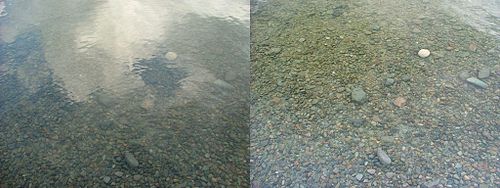
11: An example of looking at shallow water, without (left) or with (right) a polarization filter. Reflection Polarizer2, by Amithshs, Wikimedia Commons, public domain.

How electromagnetic radiation is created

Now that we know how to quantify different properties of electromagnetic radiation, we will take a brief look at how it is created in the first place. Physicists say that EMR is produced when charged particles are accelerated, this happens all the time, so it is not helpful in the context of remote sensing. Of greater use in remote sensing, we can look at the spectral radiance created by a surface, i.e. the amount of radiation created and its distribution across different wavelengths. This depends primarily on the temperature of the surface, and is neatly described for blackbodies by Planck’s Law:

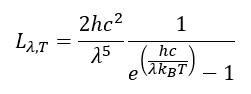
In Planck’s Law, L_λ,T is radiance, with the subscripts indicating that it is dependent on wavelength and temperature (of the surface). h is Planck’s constant, c is the speed of light in a vacuum, λ is wavelength, k_B is the Boltzmann constant (not to be confused with the Stefan-Boltzmann constant!), T is the surface temperature in degrees Kelvin. While Planck’s Law can initially look intimidating, keep in mind that h, c and k_B are all constants, so all it says is that the radiance emitted by a surface (L_λ,T) can be calculated from the temperature (T) of that surface for a given wavelength (λ).

To take a look at the result of Planck’s Law, you can imagine an object with a certain surface temperature, like the Sun whose temperature is roughly 5800K, and calculate the radiance it emits at, say, 400nm, by simply plugging the temperature and wavelength into the equation. You can then repeat for 401nm, 402nm, and so on, to produce what is called a Planck curve. An example of several Planck curves is provided in Figure 12. Note that very little radiation is produced at very short wavelengths (e.g. 0-200nm), and each curve has a distinct peak that shows the wavelength at which the maximum amount of energy is emitted. The location of this peak can be calculated using Wien’s Law, which is based on Planck’s Law, and which says that the wavelength of peak emission (λ_max) can be calculated as λ_max=bT, where b is Wien’s displacement constant: 2,897,767 nm K. For the Sun, this comes to approximately 500 nm, which is blueish-greenish light.

One important note on Planck’s Law is that it applies to blackbodies, which are imaginary entities that are defined as perfect absorbers and perfect emitters. While real-world objects, like the Sun and the Earth, are not blackbodies, they come close enough to being blackbodies most of the time for Planck’s Law to be a useful approximation that can be used to quantify their emission of electromagnetic radiation. How close or far a surface is to being a blackbody is defined by its emissivity, which is the amount of radiance produced at a given wavelength compared to that which would be produced by a blackbody. Natural materials tend to have high emissivity values, in the range of 0.98-0.99 (water), 0.97 (ice), and 0.95-0.98 (vegetation). However, some natural materials can have low emissivity, like dry snow (appr. 0.8) or dry sand (0.7-0.8). What this means, for example, is that dry snow at a given temperature only produces 80% of the radiance that it should according to Planck’s Law. A further complication is due to the fact that emissivity changes with wavelength, but that‘s a bridge to cross another time.

Planck’s Law can be used to determine the temperature of a surface whose spectral radiance is measured. This is done simply by inverting the equation to isolate temperature:

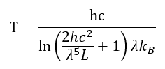
While actual determination of the Earth’s surface temperature from space-based measurement of (spectral) radiance is slightly more complicated because both emissivity and the influence of the atmosphere need to be taken into account, the inversion of Planck’s Law as outlined above is the basic principle upon which such mapping rests.

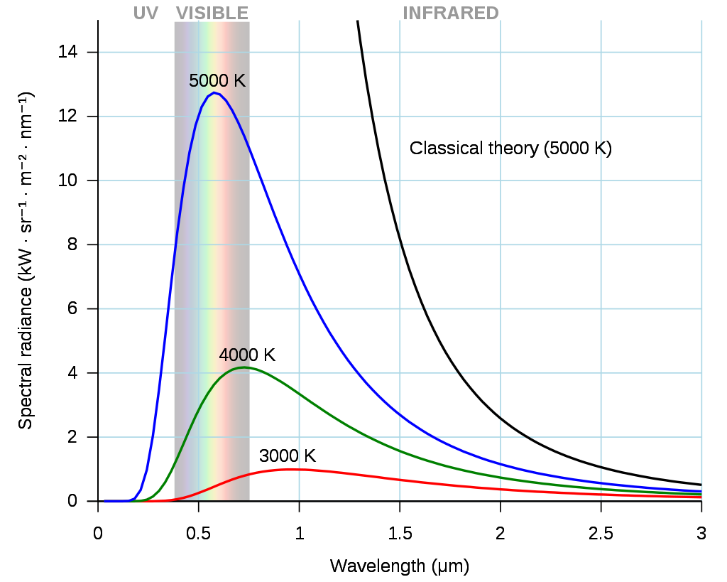
12: Example of three Planck curves, for surfaces at 3000-5000 degrees Kelvin. Black body by Darth Kule, Wikimedia Commons, public domain.