9.1: Introduction

Module 9

Geologic Time

Figure 1. There is about a 1.2 billion year gap in the rock – that is the Great Unconformity. Clear Creek trail, Grand Canyon National Park

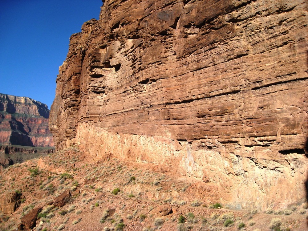
Introduction

Geologic time is immense. The Earth has existed for approximately 4.6 billion years, and many geologic processes occur over timescales of millions of years. Given that it is unusual for a person to live over 100 years, grasping the immensity of geologic time is challenging. In this module, you will learn about ways in which relative time can be determined, and about techniques that can be used to estimate numerical ages of Earth materials. You will also learn about the units that are used to measure geologic time.

The amount of time that is involved in the carving of the landscape, the formation of rocks, or the movement of the continents is an important scientific question. Different hypotheses about the age of the Earth can essentially change our perspective of the workings of geologic events that molded the Earth. If the geologic time is relatively short then catastrophic events would be required to form the features we see on the surface of the Earth, whereas a vast amount of time allows the slow and steady pace that we can easily observe around us today.

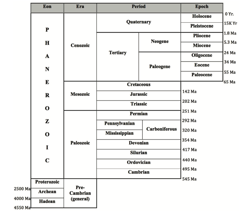
Geologists have used many methods to reconstruct geologic time and mapping the major events in Earth’s history as well as their duration. Scientists studying rocks were able to piece together a progression of rocks through time to construct the Geologic Time Scale below. This time scale was constructed by lining up in order rocks that had particular features such as rock types, environmental indicators, or fossils. Scientists looked at clues within the rocks and determined the age of these rocks in a comparative sense. This process is called relative dating, which is the process of determining the comparative age of two objects or events. For example, you are younger than your parents. It doesn’t matter your age or your parents’ age, as long as you can establish that one is older than the other. As time progressed, scientists discovered and developed techniques to date certain rocks, as well as the Earth itself. They discovered the Earth was billions of years old (4.54 billion years old) and put a time frame to the geologic time scale. This process is called absolute dating, which is the process of determining the exact amount of time that has passed since an object was formed or an event occurred.

Figure 2. The geologic time scale. “Ma” stands for millions of years [ago], while “K Yr” stands for thousands of years [ago].

Both absolute and relative dating have advantages and are still frequently used by geologists. Dating rocks using relative dating allows a geologist to reconstruct a series of events cheaply, often very quickly, and can be used out in the field on a rocky outcrop. Relative dating also can be used on many different types of rocks, where absolute dating is restricted to certain minerals or materials. However, absolute dating is the only method that allows scientists to place an exact age to a particular rock.

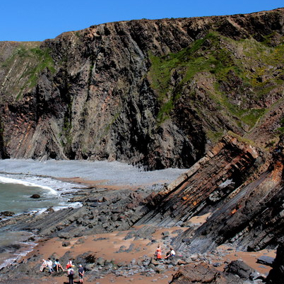
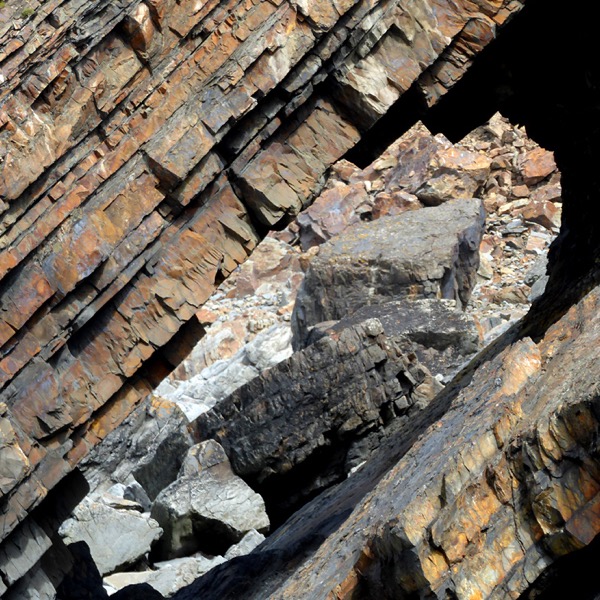
Select an image to view larger

Figure 3. These folded and crumpled strata are in the cliffs just to the north of Hartland Quay, Devon, UK. The rocks of Hartland Quay are the remains of a mountain range. Sedimentary rocks were deposited in a shallow sea during the Carboniferous period – about 320 million years ago. The layers are sequences of shales and mudstones representing the remains of sub-marine “avalanches” of sediments called turbidites. At the same time as the sands and mudstones were being deposited at Hartland, coals were being deposited in swamps, forming the South Wales coalfields. Plate tectonics caused the collision of two super continents with Hartland Quay in the middle. Devon was at the southern margin of a super-continent called Laurasia, which collided with the super-continent Pangaea – to the South. As these two mega-continents collided during the Variscan Orogeny the rocks at Hartland Quay were buckled and folded, producing the spectacular chevron shaped folds exposed in the cliffs today. The top surface was then eroded flat. – Simon Jones

Figure 4. Close up image of the layers of sediment at Hartland Quay of Figure 1.

Figure 5. Santa Elen Canyon, Big Bend, Texas. From 500 million year old rocks at Persimmon Gap to modern-day windblown sand dunes at Boquillas Canyon, geologic formations in Big Bend demonstrate amazingly diverse depositional styles over a vast interval of time.

Figure 6. Acasta Gneiss, Northwest Territory, Canada. At 3.96 billion years old, this gneiss is one of the oldest known Earth rocks. The Earth is 500 million years older still, but little record of that early time has survived our planet’s geologic activity.

Figure 7. The Earth is very old — 4.5 billion years or more according to recent estimates. Most of the evidence for an ancient Earth is contained in the rocks that form the Earth’s crust. The rock layers themselves — like pages in a long and complicated history — record the surface-shaping events of the past, and buried within them are traces of life –the plants and animals that evolved from organic structures that existed perhaps 3 billion years ago. Also contained in rocks once molten are radioactive elements whose isotopes provide Earth with an atomic clock. Within these rocks, ‘parent’ isotopes decay at a predictable rate to form ‘daughter’ isotopes. By determining the relative amounts of parent and daughter isotopes, the age of these rocks can be calculated. Thus, the results of studies of rock layers (stratigraphy), and of fossils (paleontology), coupled with the ages of certain rocks as measured by atomic clocks (geochronology), attest to a very old Earth!

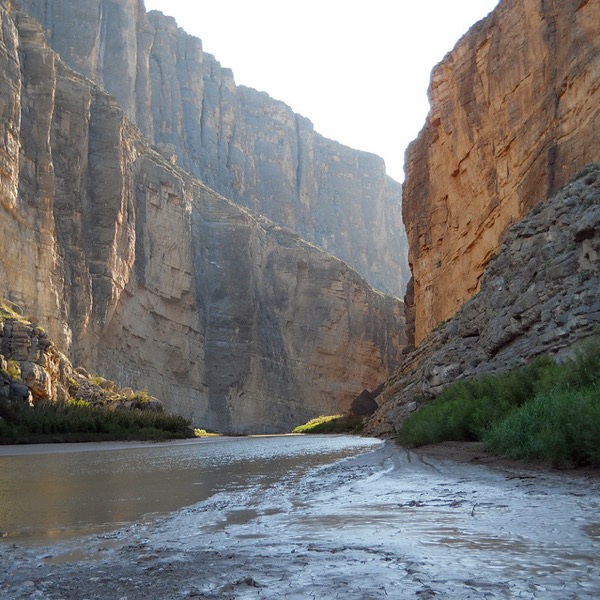
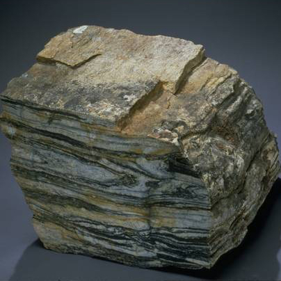
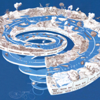
Module Objectives

At the completion of this module you will be able to:

1. Apply basic geological principles to the determination of the relative ages of rocks.
2. Explain the difference between relative and absolute age-dating techniques.
3. Summarize the history of the geological time scale and the relationships between eons, eras, periods, and epochs.
4. Understand the importance and significance of unconformities.
5. Describe the applications and limitations of using isotopes, tree rings, and magnetic data for geological dating.

---

Activities Overview

See the Schedule of Work for dates of availability and due dates.

Be sure to read through the directions for all of this module’s activities before getting started so that you can plan your time accordingly. You are expected to work on this course throughout the week.

Read

Physical Geology by Steven Earle

• Chapter 8 (Measuring Geologic Time)

Module 9 Assignment: Relative Dating and Cross Cutting Relationships

10 points

After you complete the reading, you can start working on Module 9 Assignment – Relative Dating and Cross Cutting Relationships

Module 9 Quiz

10 points

Module 9 Quiz has 10 multiple-choice questions and is based on the content of the Module 9 readings and Assignment 9.

The quiz is worth a total of 10 points (1 points per question). You will have only 10 minutes to complete the quiz, and you may take this quiz only once. Note: that is not enough time to look up the answers!

Make sure that you fully understand all of the concepts presented and study for this quiz as though it were going to be proctored in a classroom, or you will likely find yourself running out of time.

Keep track of the time, and be sure to look over your full quiz results after you have submitted it for a grade.

Your Questions and Concerns…

Please contact me if you have any questions or concerns.

General course questions: If your question is of a general nature such that other students would benefit from the answer, then go to the discussions area and post it as a question thread in the “General course questions” discussion area.

Personal questions: If your question is personal, (e.g. regarding my comments to you specifically), then send me an email from within this course.