1.9: Lab 9 - Climate Patterns

This lab contains potentially inaccessible interactive resources. Please work with your instructor and local campus resources to identify accommodations for these resources.

Learning Objectives

• Interpret climographs.
• Explain the main controls on climate.
• Compare climates using the Köppen–Geiger classification system.
• Apply an understanding of climate types to California and your local area.
• Analyze temporal and spatial climate shifts.

Introduction

Climate patterns are long-term atmospheric conditions that influence life on Earth. Typically, scientists use thirty years of weather data, such as average monthly temperatures and precipitation, to classify a location’s climate. Our climate influences our day-to-day actions and impacts our resource consumption in terms of energy usage for the heating and cooling of our homes and workplaces. Our behaviors are influenced by climate, as well:

➢ Do you own a raincoat and carry an umbrella most of the year?

➢ Do you work outdoors in the early morning to avoid the extreme heat of the afternoon sun during the summer months?

➢ Do you carry snow chains for your car tires in the winter months?

In this lab, you will learn the major variables that determine a location’s climate, how climates are classified, and how these climate classifications change over time.

Part A. Controls on Climate

Why is New York City hot and humid in the summer? Why is Seattle known for rain? Why does San Diego experience so many days of sunshine? To answer these questions, you must understand the major variables that influence a location’s climate—the long-term weather conditions. What you have learned so far in this physical geography laboratory course will help you to understand these variables.

Climograph Interpretation

Before we introduce these variables, let’s learn how to interpret a climograph. A climograph is a helpful chart that graphs average monthly precipitation and temperature. A blank climograph is shown in Figure 9.1. The months are shown along the x-axis, starting with January (J) on the far-left and going through to December (D) on the far-right. Average monthly precipitation is on the left y-axis, shown in centimeters. For reference, one inch is 2.54 centimeters. So, a location that receives 10 inches of rain on average in January receives 25.4 centimeters of rain. Average monthly temperature is shown on the right y-axis, shown in degrees Celsius. For reference, 32°F (freezing/melting point of water) is 0°C, 70°F is 21.1°C, and 100°F is 37.8°C.

Pin It! Metric Conversions

The scientific community uses the metric system, so the climographs and climate classification data in this lab are shown in metric units. Try to relate the American units that you already know (such as degrees Fahrenheit and inches) to their metric equivalents. Here are some examples to help you make the connection between the American units that you know and their metric equivalents:

➢ 50°F is 10°C, 70°F is ~21°C, and 90°F is ~32°C.

➢ 1 inch is 2.54 centimeters, 5 inches is 12.7 centimeters, and 10 inches is 25.4 centimeters.

Figure 9.1: Blank Climograph. Figure by Scott Crosier is licensed under CC BY-NC-SA 4.0

In order to complete the climograph, you need the average monthly precipitation and temperature for a location. Table 9.1 provides this data, which we will use to create an example climograph.

Table 9.1: Climograph Data for a Location

Month	Average Precipitation (cm)	Average Temperature (°C)
January	5.9	22.9
February	5.1	22.8
March	5.1	23.6
April	1.6	24.5
May	1.6	25.4
June	0.7	26.8
July	1.3	27.3
August	1.4	27.7
September	1.8	27.5
October	4.7	26.7
November	6.1	25.3
December	8.2	23.8

In this example, we’ll first plot the precipitation data from Table 9.1 on the climograph using a bar graph for each month. As you will note in Figure 9.2 below, the blue bars represent average monthly precipitation. Note: the blue color is arbitrary; climographs may show precipitation in green or another color.

Figure 9.2: Climograph with Only Precipitation Plotted. Figure by Waverly Ray is licensed under CC BY-NC-SA 4.0

The next step to create the example climograph is to plot the temperature data from Table 9.1. We have used an orange line to represent average monthly temperature as shown in Figure 9.3. Note: the orange color is arbitrary; climographs may show temperature in red or as another color.

Figure 9.3: Climograph with Precipitation and Temperature Plotted. Figure by Waverly Ray is licensed under CC BY-NC-SA 4.0

Exercise \(\PageIndex{1}\)

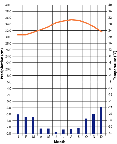
1. Refer to Figure 9.3. How does the climograph help us understand the location’s climate? Create a list of what you can determine from the climograph. Here are two questions to help you write your response: does the location’s temperature fluctuate or is it within about a 15°C temperature range throughout the year? When is the rainy season? (This is when precipitation levels increase).

Five Major Controls on Climate

Now that you are familiar with climographs, let’s take a look at the variables that influence a location’s climate—we call these variables climatic controls (or controls on climate). These variables explain why a location might (or might not) have temperatures that fluctuate greatly throughout the year, why the location might have a rainy season, etc. While we will look at each variable individually, it’s important to remember that these variables may interact to influence a particular location in a unique way.

Latitude

The first and most important variable that influences a location’s climate is latitude. Low latitudes (closer to the equator) receive higher total insolation year-round than higher latitudes (closer to the poles). So, locations at tropical latitudes show little temperature changes throughout the year compared to higher latitudes. Locations at middle and high latitudes show a wider range in temperatures because of the tilt of the Earth, which influences insolation amounts and daylight hours throughout the year.

Exercise \(\PageIndex{2}\)

2. Compare the two climographs shown below (Figure 9.4). Does climograph A (on the left) or B (on the right) represent a location at 61° North latitude? Explain your response in at least one sentence.

Figure 9.4: Climograph Examples A (on left) and B (on right). Figure by Waverly Ray is licensed under CC BY-NC-SA 4.0

Continentality

The second variable that influences a location’s climate is continentality. This refers to whether a location is located along a coastline or is inland. Variations in climate are due in part to land-water contrasts. Land and water react differently to insolation. In general, land heats up and cools off faster than water does due to its specific heat. A location in the interior of a continent will be warmer in the summer and cooler in winter than a maritime (coastal) location at the same latitude. So, maritime regions have a lower annual temperature range than continental regions.

Exercise \(\PageIndex{3}\)

3. Compare the two climographs shown below (Figure 9.5). Both locations are near 40° North latitude. Does climograph C (on the left) or D (on the right) represent a maritime location? Explain your response in at least one sentence.

Figure 9.5: Climograph Examples C (on left) and D (on right). Figure by Waverly Ray is licensed under CC BY-NC-SA 4.0

Wind Patterns and Air Masses

Wind patterns and air masses also influence a location’s climate. Here are several examples of their influence:

➢ In midlatitudes in the Northern Hemisphere, the dominant winds are the westerlies. These winds travel from west to east and bring seasonal warmth or coolness to eastern locations.

➢ Monsoons are the seasonal reversal of winds that bring very high precipitation levels around June through August in South Asia.

➢ Locations influenced by maritime tropical air masses will have higher levels of precipitation and temperature than locations influenced by polar continental air masses.

Exercise \(\PageIndex{4}\)

4. Compare the two climographs shown below (Figure 9.6). Both locations are found at 21° North latitude. Why does the location depicted by climograph E (on the left) have higher levels of precipitation when compared to climograph F (on the right)? Explain your response in at least one sentence.

Figure 9.6: Climograph Examples E (on left) and F (on right). Figure by Waverly Ray is licensed under CC BY-NC-SA 4.0

Ocean Currents

Ocean currents also influence a location’s climate. The major surface ocean currents move warm water from equatorial regions toward polar regions and they bring cool water from the polar regions to equatorial regions. As a result, ocean circulation is a significant mechanism of global heat transfer.

The surface ocean current map (Figure 9.7) shows cold currents in blue and warm currents in red. Notice that warm currents are found in equatorial locations. Recall from a previous lab that surface ocean currents are driven by global atmospheric circulation. This explains why many west coasts of continents have cold currents while east coasts have warm currents. Warm currents bring warmer temperatures and higher levels of precipitation compared to cold currents.

Figure 9.7: Map of Surface Ocean Currents. Used by permission. Dataset source: Laura Walker, Program Manager, O'Neill Sea Odyssey

Exercise \(\PageIndex{5}\)

5. Both locations shown by their climographs in Figure 9.8 are near 33° latitude. Based on the temperature curves on both climographs, how do you know if these locations are in the northern or southern hemisphere? Explain your response in at least one sentence.

5. Compare the two climographs shown below (Figure 9.8). Which location is near a warm surface ocean current? Explain your response in at least one sentence.

Figure 9.8: Climograph Examples G (on left) and H (on right). Figure by Waverly Ray is licensed under CC BY-NC-SA 4.0

Elevation

The final important control on climate is elevation. As you learned when you studied orographic lifting, under normal conditions temperatures decrease between 6 and 10 degrees Celsuis for every 1,000 meters that the elevation increases. Locations on the windward side of mountains receive precipitation and locations on the leeward side of mountains are in the rainshadow.

Exercise \(\PageIndex{6}\)

7. Compare the two climographs shown below (Figure 9.9). Both locations are found at 48° North latitude. Which climograph represents a location in the rainshadow of a mountain? Explain your response in at least one sentence.

Figure 9.9: Climograph Examples I (on left) and J (on right). Figure by Waverly Ray is licensed under CC BY-NC-SA 4.0

Pin It! The Five Main Controls on Temperature

Remember the five climatic controls when analyzing a location’s climate: latitude, continentality, wind patterns and air masses, ocean currents, and elevation.

Exercise \(\PageIndex{7}\)

8. Apply What You Learned: Match climographs B through J (shown in Figures 9.4, 9.5, 9.6, 9.8, and 9.9 above) to their real-world locations shown in Table 9.2. To complete Table 9.2, use a globe, atlas, or the internet to find where each city is located, the city’s elevation, and whether the city is maritime (coastal) or continental (inland of a continent). Tips:

➢ Remember to indicate N or S for the latitudes of each city.

➢ Complete the southern hemisphere locations first (their climographs should be distinct from the northern hemisphere locations in terms of temperature).

➢ Several questions above indicate the latitudes of the climographs so you can use this information to narrow down the cities.

Table 9.2: City-Climograph Matching

City	Latitude (to the nearest degree)	Elevation (indicate feet or meters)	Maritime or Continental	Climograph Letter (Select from B through J)	List the Major Climatic Controls at this City:
Anchorage, Alaska
Denver, Colorado
Eureka, California
Hanoi, Vietnam
Honolulu, Hawai’i
Perth, Australia
Seattle, Washington
Spokane, Washington
Sydney, Australia

Part B. Climate Classification

Understanding the major variables that influence climate helps explain why a particular location experiences the climate that it does. In order to understand climate patterns, we need to classify climates. This helps us to know what locations experience similar climatic conditions.

The Köppen–Geiger climate classification system is one of the most commonly used methods to classify a location’s climate. It was first developed in the late 1800s and revised through the early 1900s. This climate classification system uses average monthly temperature and precipitation data to classify climates into five main groups:

➢ Tropical climates are humid with monthly average temperatures of at least 18°C (64.4°F). Tropical climates are designated with an “A”.

➢ Dry climates are found at locations with little precipitation, which causes evaporation to exceed precipitation and results in water deficiencies throughout the year. Dry climates are designated with a “B”.

➢ Temperate climates have at least one month with an average temperature higher than 10°C (50°F) and a coldest month with an average temperature between 0°C (32°F) and 18°C (64.4°F). Temperate climates are designated with a “C”.

➢ Continental climates have at least one month with an average temperature lower than 0°C (32°F) and at least one month with an average temperature higher than 10°C (50°F). Continental climates are designated with a “D”.

➢ Polar climates have an average monthly temperature below 10°C (50°F). Polar climates are designated with an “E”.

Exercise \(\PageIndex{8}\)

9. Use Your Critical Thinking Skills: Why do you think average monthly temperatures were used to classify climates? Explain your response in one to two sentences.

10. Use Your Critical Thinking Skills: Why do you think particular temperatures were used to classify climates? In other words, why would the creators of the Köppen–Geiger climate classification system use 0°C (32°F), 10°C (50°F), or 18°C (64.4°F) to divide the climate types? Explain your response in one to two sentences.

The world map below (Figure 9.10) shows the five major climate types.

Figure 9.10: Map of Major Climate Classification Types (1901-2010). Figure by Waverly Ray based on data available from http://hanschen.org is licensed under CC BY-NC-SA 4.0

Exercise \(\PageIndex{9}\)

11. Refer to Figure 9.10. List three observations that you can make based on the spatial patterns presented on the map. These observations could be something that is unexpected or surprising.

Within each of the five main climate types, there are further subdivisions to classify climates. Figure 9.11 is a map that shows all of these climate classifications. An enlarged version of this map is available in Appendix 9.1.

Figure 9.11: Climate Classification Map (1901-2010). Figure by Waverly Ray based on data available from http://hanschen.org is licensed under CC BY-NC-SA 4.0

Exercise \(\PageIndex{10}\)

12. Refer to Figure 9.11 (or Appendix 9.1). List three observations that you can make based on the spatial patterns presented on the map. These observations could be something that is unexpected or surprising.

A Climates

For A climates (tropical climates), a second letter is added. It’s important to note that monsoons are the seasonal reversal of winds that bring tremendous amounts of precipitation to much of South and Southeast Asia. Also note that a savanna is a grassland found in the tropics and subtropics.

➢ Af indicates year-round precipitation. This is a Tropical Rainforest climate.

➢ Am indicates monsoonal precipitation. This is a Tropical Monsoon climate.

➢ Aw indicates a savanna climate with a relatively dry winter. This is a Tropical Wet Savanna climate.

➢ As indicates a savanna climate with a relatively dry summer. This is a Tropical Dry Savanna climate.

Exercise \(\PageIndex{11}\)

13. Refer to Figure 9.11 above. Describe the spatial distribution for the A climate types. (Where are the A climates found?)

14. Apply What You Learned: Why do you think the southeast Asian islands have a Tropical Rainforest climate but the continental parts of Southeast Asia and South Asia have both the Tropical Monsoon and the Tropical Savanna climates? Explain your response in one to two sentences.

15. The Lion King film is set in the Tropical Savanna of Africa. Estimate the percentage of the African continent that have this climate type. (Do you think the Tropical Savanna climate is one-quarter, one-half, or three-quarters of the continent?)

B Climates

For B climates (dry climates), second and third letters are added. If W is the second letter, then it represents a desert location. If S is the second letter, then it represents a steppe (midlatitude grassland) location. If the third letter is h, this represents a relatively hot arid location. If the third letter is k, this represents a relatively cold air location.

➢ BWh is a Hot Desert climate.

➢ BWk is a Cold Desert climate.

➢ BSh is a Hot Semi-Arid climate.

➢ BSk is a Cold Semi-Arid climate.

Exercise \(\PageIndex{12}\)

16. Refer to Figure 9.11 above. Describe the spatial distribution for the B climate types. (Where are the B climates found?)

17. What is the latitude that intersects much of the land with the B climate types in the northern and southern hemispheres? Hint: this latitude is where subtropical high pressure systems are dominant.

C Climates

For C climates (temperate climates), second and third letters are added. If w is the second letter, then it represents a location with a relatively dry winter. If f is the second letter, there is not a dry season at this location. If s is the second letter, then it represents a location with a relatively dry summer. If a is the third letter, then it represents a location with a relatively hot summer. If b is the third letter, then it represents a location with a relatively warm summer. If c is the third letter, then it represents a location with a relatively cool summer. Here are some of the C climate types:

➢ Cfa is a Humid Subtropical climate.

➢ Cfb is a Marine West Coast climate with a relatively warm summer.

➢ Cfc is a Marine West Coast climate with a relatively cool summer.

➢ Cwa is a Humid Subtropical climate with a dry winter.

➢ Csa is a Hot-Summer Mediterranean climate.

➢ Csb is a Warm-Summer Mediterranean climate.

➢ Csc is a Cold-Summer Mediterranean climate.

Exercise \(\PageIndex{13}\)

19. Which climate type is most common in the southeastern United States?

20. The Cfb and Cfc Marine West Coast climates are not only found on the west coasts of continents. Where is this climate type found when it is not on a west coast of a land mass?

21. The Csa, Csb, and Csc Mediterranean climates are not only found in the Mediterranean regions of Africa, Southwest Asia, and Europe. Where is this climate type found outside of the Mediterranean region?

D Climates

For D climates (continental climates), second and third letters are added. It utilizes the same second and third letter designations as the C climates, with an additional letter option for the third letter. When the third letter is d, this designates a location with a very cold winter. Here are some of the D climate types:

➢ Dfa is a Hot-Summer Continental climate.

➢ Dfb is a Warm-Summer Continental climate.

➢ Dfc is a Subarctic climate.

➢ Dfd is an Extremely Cold Subarctic climate.

➢ Dwa is a Hot-Summer Humid Continental climate.

➢ Dwb is a Warm-Summer Humid Continental climate.

➢ Dwc is a Subarctic Humid Continental climate.

➢ Dwd is an Extremely Cold Humid Subarctic climate.

Exercise \(\PageIndex{14}\)

22. Refer to Figure 9.11 above. Describe the spatial distribution for the D climate types. (Where are the D climates found?)

E Climates

There are three types of E (polar climates):

➢ ET is a Tundra climate.

➢ EF is an Ice Cap climate.

➢ EM is a Polar Marine climate.

Exercise \(\PageIndex{15}\)

23. Refer to Figure 9.11 above. Describe the spatial distribution for the E climate types. (Where are the E climates found?)

Simplified Guide to Climate Classification

In describing each of the five main climate classification categories, we have left out the details of what is meant by the descriptions such as warm summer and dry winter. In order to understand how the climates are actually classified into the different categories, use Figure 9.12, which is a simplified guide to climate classifications.

Figure 9.12: Simplified Guide to Climate Classifications. Figure by Scott Crosier is licensed under CC BY-NC-SA 4.0

Next, you will use the Simplified Guide to Climate Classifications (Figure 9.12) and data from four example locations to identify each location’s climate type.

Exercise \(\PageIndex{16}\)

24. Use Figure 9.12 above and the data provided in Table 9.3 below to find the climate classification for the example 1 location. What climate classification best fits this location?

Table 9.3: Example 1 Location Climate Data

Month	Average Precipitation (cm)	Average Temperature (°C)
January	1.8	-9.6
February	1.7	-7.7
March	1.6	-3.6
April	1.0	2.6
May	1.8	8.7
June	2.6	13.2
July	4.8	14.9
August	7.3	13.8
September	6.5	9.1
October	5.0	1.1
November	2.6	-6.2
December	3.1	-8.0
Mean Annual	3.3	2.4
Annual Total	39.8	n/a

25. Use Figure 9.12 above and the data provided in Table 9.4 below to find the climate classification for the example 2 location. What climate classification best fits this location?

Table 9.4: Example 2 Location Climate Data

Month	Average Precipitation (cm)	Average Temperature (°C)
January	38.5	27.1
February	31.0	27.3
March	10.0	28.4
April	25.8	28.8
May	13.3	29.0
June	8.3	28.1
July	3.1	28.7
August	3.4	28.5
September	2.9	29.3
October	3.3	29.1
November	7.5	28.1
December	8.4	28.5
Mean Annual	13.8	28.4
Annual Total	165.5	n/a

26. Use Figure 9.12 above and the data provided in Table 9.5 below to find the climate classification for the example 3 location. What climate classification best fits this location?

Table 9.5: Example 3 Location Climate Data

Month	Average Precipitation (cm)	Average Temperature (°C)
January	3.7	3.1
February	3.4	5.3
March	3.7	10.3
April	2.8	16.4
May	1.5	22.1
June	0.3	27.5
July	0.3	30.4
August	0.2	29.2
September	0.1	25.4
October	1.4	18.5
November	2.1	11.6
December	3.6	5.6
Mean Annual	1.9	17.1
Annual Total	23.1	n/a

27. Use Figure 9.12 above and the data provided in Table 9.6 below to find the climate classification for the example 4 location. What climate classification best fits this location?

Table 9.6: Example 4 Location Climate Data

Month	Average Precipitation (cm)	Average Temperature (°C)
January	10.6	10.2
February	10.3	11.6
March	7.5	12.7
April	3.3	13.8
May	1.2	15.3
June	0.3	16.8
July	0.0	17.6
August	0.1	18.1
September	0.4	18.2
October	2.4	16.6
November	6.0	13.2
December	10.2	10.3
Mean Annual	4.4	14.5
Annual Total	52.3	n/a

California’s Climate Types

Four of the five major Köppen climate types are present in California (Figure 9.13). In parts of the Great Basin desert, Mojave desert, and the Colorado portion of the Sonoran desert found in California, there is a dry (B) climate. The Mediterranean climate types (Cs) are found along coastal California and the Channel Islands. Cold continental (D) and polar (E) climates are found at higher elevations in the Sierra Nevada Mountains. The state’s topography and geomorphic provinces are shown in Figure 9.14. (Topography refers to the elevation changes and features on land; geomorphic provinces are regions that have similar geographic features).

Figure 9.13: California Climate Map. Figure by Adam Peterson is licensed under CC BY-SA 4.0

Figure 9.14: California Topography and Geomorphic Provinces Map. Figure by Ssalonen is licensed under CC BY-SA 3.0

Exercise \(\PageIndex{17}\)

28. Compare California’s climate map (Figure 9.13) to the California topography map (Figure 9.14). What are the peak elevations where an ET climate is found?

29. The San Joaquin Valley is one of the most productive agricultural areas in the world.

​​​​​​​

1. What climate type is found there? Tip: first, locate the San Joaquin Valley on Figure 9.14 (at about 37°N) then identify the climate type shown in Figure 9.13.

2. Use Your Critical Thinking Skills: What are the implications for the irrigation needs in the San Joaquin Valley? Explain your response in two to three sentences.

Shifting Climate Patterns

As you learned earlier in the lab, at least thirty years of precipitation and temperature data are used to classify a location’s climate. As climates change across the globe, it makes sense that maps like the ones shown in Figure 9.11 and 9.13 above will need to be updated. Scientists actively research how climate classification patterns have changed over time and predict how these patterns will change in the future. The next lab in this course will go into more detail to explain why climates are changing. For now, let’s explore one dynamic online map that shows historical shifting climate patterns and predictions based on data from the Institute for Veterinary Public Health, Climatic Research Unit (CRU), Global Precipitation Climatology Centre (GPCC), German Weather Service, University of East Anglia, Tyndall Centre for Climate Change Research, and the Intergovernmental Panel on Climate Change.

Step 1

Go to the Koppen-Geiger Observed and Predicted Climate Shifts website.

Step 2

Click on the legend icon. (This is on the upper-left of the window. If you hover over the icons, it is the one that says Show Map Legend).

Step 3

Scroll downwards so that you are familiar with the colors used to classify the climate types.

Step 4

Below the map, click on the blue triangle, which will start the map animation. Notice that the animation begins at 1900 and goes to 2100.

Step 5

Replay the animation in order to answer the following questions.

Exercise \(\PageIndex{18}\)

30. What is the first year that you notice a large change in the maps?

30. In two to three sentences, describe how the climate pattern is predicted to change in North America from 2000 to 2100.

30. Globally, which climate types show the most change from 2000 to 2100?

Part C. Synthesis: Your Local Climate

What does a climograph look like for your location? What variables influence your local climate? In this part of the lab, you will find monthly average precipitation and temperature data for your location (or for a location near you), create a climograph, determine the climate type, and then identify the controls on climate at this location.

Exercise \(\PageIndex{19}\)

33. Search the internet to find the average monthly precipitation and temperature data for your location (or for a location near you). Be sure to convert average precipitation to centimeters (cm) and average temperature into degrees Celsius (°C). Complete the table below with this data (Table 9.7). Your instructor may direct you to online resources that provide this information, or you may follow the steps below for data for selected cites from the U.S. Climate Data website.

Step 1

Go to the U.S. Climate Data website.

Step 2

In the search box, type in your location (or a location near to you). Select your location if a drop-down menu appears.

Step 3

Change the data from American to metric units. In the upper-right corner, click the gear icon to select °C. Tip: this step is very important.

Step 4

If the monthly average precipitation data is shown in millimeters (mm), convert to centimeters (cm) by dividing by 10. For example, if the average precipitation in January is 50.29 millimeters then divide this number by 10, which equals 5.029. Tip: round the data to the nearest hundredth decimal point, so 5.029 centimeters would be recorded as 5.03 on Table 9.7.

Add the monthly average precipitation data to Table 9.7.

Step 5

The table shows average high temperatures and average low temperatures, but you will need average temperature to complete Table 9.7. To calculate average temperature, use this formula:

Monthly Average High Temperature + Monthly Average Low Temperature = Monthly Average T.

2

For example, if the January average high temperature is 18.3°C and the monthly average low temperature is 9.4°C, then add 18.3°C plus 9.4°C, which equals 27.7°C. Then, divide 27.7°C by two, which equals 13.85°C (the January monthly average temperature). Tip: round the data to the nearest tenth decimal point, so 13.85°C would be recorded as 13.9°C on Table 9.7.

Exercise \(\PageIndex{20}\)

Add the monthly average temperature data to Table 9.7

Table 9.7: Local Precipitation and Temperature Data

Month	Average Precipitation (cm)	Average Temperature (°C)
January
February
March
April
May
June
July
August
September
October
November
December
Mean Annual
Annual Total

34. Use Your Critical Thinking Skills: The Weather Channel website does not disclose how the average precipitation and temperature are calculated. It could be a 30-year average, a 10-year average, or something else. How would the length of time used to calculate the average affect your analysis of the data? More broadly, what are the concerns with using datasets if the source does not disclose its methods of calculations? Your response should be two to three sentences in length.

35. Following the example shown in Figure 9.3, graph your location’s precipitation and temperature data on the blank climograph (Figure 9.15). Use the left y-axis to graph precipitation data as a bar graph and use the right y-axis to graph temperature data as a line graph.

Figure 9.15: Blank Climograph. Figure by Scott Crosier is licensed under CC BY-NC-SA 4.0

36. Refer to California’s Climate Map (Figure 9.13). What is the climate type at your location?

37. Use your location’s data from Table 9.7 and the simplified guide to climate classification (Figure 9.12) to determine your location’s climate type. Based on the simplified guide, what is your location’s climate type?

38. Use Your Critical Thinking Skills: Are your answers to questions 36 and 37 the same? If not, what reasons might explain why the map and the simplified guide provided different answers?

39. Refer to Figure 9.14. What geomorphic province is your location in?

40. List the major climatic controls at your location. Tip: the major climatic controls are latitude, continentality, wind patterns and air masses, ocean currents, and elevation. Be sure to discuss the specifics of each climatic control that influences the local climate at your location. For example, if a wind pattern influences the local climate, be sure to identify the name or type of wind, such as the westerlies.

41. Apply What You Learned: Considering how climate patterns are shifting globally, do you anticipate that the climate type at your location will change by 2100? Explain your response in at least two sentences.

Part D. Wrap-Up

Consult with your geography lab instructor to find out which of the following wrap-up questions you should complete. Attach additional pages to answer the questions as needed.

Exercise \(\PageIndex{21}\)

42. What is the most important idea that you learned in this lab? In two to three sentences, explain the concept and why it is important to know.

43. What was the most challenging part of this lab? In two to three sentences, explain why it was challenging. If nothing challenged you in the lab, write about what you think challenged your classmates.

44. What is one question that you have about what you learned in this lab? Write your question along with one to two sentences explaining why you think your question is important to ask.

45. Review the learning objectives on page 1 of this lab. How would you rate your understanding or ability for each learning objective? Write one sentence that addresses each learning objective.

46. Sketch a concept map that includes the key ideas from this lab. Include at least five of the terms shown in bold-faced type.

47. Create an advertisement to educate your peers on the important information that you learned in this lab. Include at least three key terms in your advertisement. The advertisement should be about half a page in size (about 4 inches by 6 inches).

48. One way to think of physical geography is that it is the study of the relationships among variables that impact the Earth's surface. Select two variables discussed in this lab and describe how they are related.

49. How does what you learned in this lab relate to your everyday life? In two to three sentences, explain a concept that you learned in this lab and how it relates to your day-to-day actions.

50. How does what you learned in this lab relate to current events?
    1. Write the title, source, and date of a news item that relates to this lab.
    2. In two to three sentences, discuss how the news item relates to what you have learned in this lab.
    3. In one to two sentences, discuss whether or not the news item accurately represents the science that you learned. Tip: consider whether or not the news item includes the complexity of the topic.

51. Search O*NET OnLine to find an occupation that is relevant to the topics presented in today's lab. Your lab instructor may provide you with possible keywords to type in the Occupation Quick Search field on the O*NET website.
    1. What is the name of occupation that you found?
    2. Write two to three sentences that summarize the most important information that you learned about this occupation.
    3. What is one question that you would want to ask a person with this occupation?

Appendix 9.1: Climate Classification Map (1901-2010)

Figure by Waverly Ray based on data available from http://hanschen.org is licensed under CC BY-NC-SA 4.0