1.4: Soil Physics

Last updated
Save as PDF

Page ID: 16608

$ \newcommand{\vecs}[1]{\overset { \scriptstyle \rightharpoonup} {\mathbf{#1}} } $ $ \newcommand{\vecd}[1]{\overset{-\!-\!\rightharpoonup}{\vphantom{a}\smash {#1}}} $$\newcommand{\id}{\mathrm{id}}$ $ \newcommand{\Span}{\mathrm{span}}$ $ \newcommand{\kernel}{\mathrm{null}\,}$ $ \newcommand{\range}{\mathrm{range}\,}$ $ \newcommand{\RealPart}{\mathrm{Re}}$ $ \newcommand{\ImaginaryPart}{\mathrm{Im}}$ $ \newcommand{\Argument}{\mathrm{Arg}}$ $ \newcommand{\norm}[1]{\| #1 \|}$ $ \newcommand{\inner}[2]{\langle #1, #2 \rangle}$ $ \newcommand{\Span}{\mathrm{span}}$ $\newcommand{\id}{\mathrm{id}}$ $ \newcommand{\Span}{\mathrm{span}}$ $ \newcommand{\kernel}{\mathrm{null}\,}$ $ \newcommand{\range}{\mathrm{range}\,}$ $ \newcommand{\RealPart}{\mathrm{Re}}$ $ \newcommand{\ImaginaryPart}{\mathrm{Im}}$ $ \newcommand{\Argument}{\mathrm{Arg}}$ $ \newcommand{\norm}[1]{\| #1 \|}$ $ \newcommand{\inner}[2]{\langle #1, #2 \rangle}$ $ \newcommand{\Span}{\mathrm{span}}$$\newcommand{\AA}{\unicode[.8,0]{x212B}}$

Sandra Brown, Asim Biswas, Jean Caron, Miles Dyck, and Bing Si

Learning Objectives

On completion of this chapter, students will be able to:

Define relationships between texture, bulk density, porosity and compaction
Describe how soils retain water and the forces driving water movement in soils
Relate water retention to soil properties, and water availability for plants
Characterize how soil water movement varies with tension and pore-size distribution
Describe the major mechanism of gas exchange in soils
List the main mechanisms of solute transport in soils and their relevance for plants
Outline soil thermal properties and factors influencing soil temperature and heat flow
Explain the effect of soil water on soil consistency

INTRODUCTION

Soil physics is the study of the solid, liquid and gaseous phases of soils, and their interactions. Soil texture, structure and bulk density reflect how soil mineral and organic particles combine to form the soil matrix and pore spaces. Pore spaces hold gases and water. Understanding soil water retention and soil water movement is crucial in determining water availability for plants and soil organisms, infiltration and drainage, runoff and erosion. Many soil nutrients are transported in the soil as solutes in soil solution. Soil aeration and gas exchange govern CO₂ emissions from the soil and O₂ availability for plants. Soil thermal properties regulate soil temperature with depth and determine how quickly (or slowly) a soil warms up in the spring. Soil strength is influenced by soil texture and water content, and determines the susceptibility of a soil to slope failure and compaction.

Understanding the impacts of land management on soil physical properties can help us develop alternative practices for managing soils in a variety of ecosystems (forest, agriculture, urban). For example, in forest operations, soils may be compacted on landings, where logs are stored and loaded onto trucks by heavy machinery. But not all soils are equally susceptible to compaction, nor will all soil types require mechanical loosening of the soil prior to tree replanting. Forest practitioners need to consider soil physical properties, such as texture and water content, as part of their assessment of the need for costly rehabilitation measures. Agriculture accounts for 85% of ammonia (NH₃) emissions in Canada (Bittman et al., 2017), in large part associated with the application of animal manure to fields. In regions with a large number of dairy and poultry farms, such as the Lower Fraser Valley in British Columbia, farmers are faced with excessive amounts of manure that are often applied to cropped fields. By understanding gas exchange in the soil-plant-atmosphere system, researchers from Agriculture and Agri-Food Canada in Agassiz were able to develop a manure spreader that injects the dairy manure into the soil between corn rows. This type of machinery reduced both air pollution (through reduction of nitrous oxide N₂O emissions) and groundwater pollution (through reduction of leaching losses of nitrates) from agricultural fields. In urban environments, the construction of houses commonly involves the removal of vegetation and topsoil from the site, and purposefully compacting the soil to reduce settling. Once construction is finished, a thin layer of topsoil is spread and seeded with grass. But the water holding capacity of this thin layer of soil is insufficient to support live grass in the summer. In the driest parts of Canada, cities such as West Kelowna in British Columbia have introduced bylaws, which require a minimum 30 cm topsoil thickness, aimed at reducing outdoor water consumption by increasing the volume of plant available water held in the soil. These are just a few examples of how soil physics can help us solve a range of soil-related environmental challenges.

SOIL IS A THREE-PHASE SYSTEM

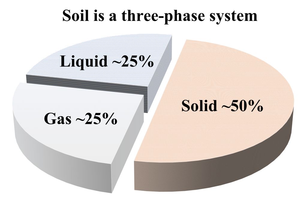
Soil is a complex three-phase system, comprised of: solids (soil mineral particles and organic matter), liquids (the soil solution: water, dissolved nutrients, chemicals, and gases), and gases (e.g., N₂, O₂, CO₂) (Figure 4.1). The magnitude and interaction among the three phases determine the behaviour and functionality of soil.

Fig_4.1-1024x672.png — Figure 4.1. Soil is a three-phase system; solid, liquid and gas. The proportion of each phase may vary, but ideally, it consists of 50% solid, 25% liquid, and 25% gas. © Asim Biswas, Univ. of Guelph is licensed under a CC BY (Attribution) license.

Solid phase

The solid phase of a soil system can be comprised of soil particles that are either mineral (i.e., rocks, stones, cobbles, gravel, sand, silt, clay) or organic (i.e., soil organic matter) in nature. Ideally, the solid phase occupies approximately 50% of the soil by volume (Figure 4.1). However, this may vary between 30 and 60% of the total soil volume based on physical conditions as well as management impacts. For example, in a sandy soil, larger mineral particles may occupy a greater volume of soil. Similarly, compaction may increase the volume of solid particles within a specified volume. While the solid mineral content is generally stable over time, the soil organic matter content may change relatively quickly. The soil mineral content consists of primary particles such as crystalline minerals (e.g., quartz, aluminosilicates) and amorphous gels (e.g., oxides, hydroxides and hydrous oxides of iron, aluminum, and manganese). These primary soil particles interact with each other. For example, amorphous gels may coat crystalline particles and form secondary particles or aggregates (as described in Chapter 2: Formation of Soil Structure). Thus, the mineral content is comprised of particles of different shapes, sizes, and chemical composition. Organic materials also contribute to the total solid phase of a soil system, but generally occupy a smaller proportion (3-5%) in mineral soils. Soil organic matter is generally comprised of live organisms, and plant and animal residues in various stages of decomposition. These organic materials can bind other mineral and organic materials together, and form secondary units (called aggregates), which also contribute to the solid phase of a soil system. The composition and surface characteristics of solids dictate the behaviour of soil and determine the interaction of solid phase with liquid (e.g., soil water, plant nutrients) and gaseous (e.g., soil air) phases.

Liquid phase

The liquid phase of a soil system consists of soil water and various nutrients, chemicals, and gases dissolved in soil water (sometimes referred to as soil solutes), forming a soil solution. Both the amount of water in soil (water quantity) and the chemical composition (water quality) contribute to the liquid phase of a soil system. Ideally, the liquid phase consists of 25% of the total volume of soil. However, it is more dynamic than the solid phase as it may vary between <1% (completely dry conditions) to approximately 50% (all spaces between the solid particles being filled with liquids). The spaces between the solid particles within a soil system are known as soil pores, and when all the pores are filled with water, the soil is considered saturated. The pores that are not filled with water within a soil system, will be filled by the gaseous phase (i.e., soil air) and thus the liquid and gaseous phases share the pore spaces within a soil system.

Gaseous phase

The gaseous phase of a soil system consists of soil air, which is a mixture of gases commonly including nitrogen (N₂), oxygen (O₂), water vapour and carbon dioxide (CO₂). Ideally, soil gases comprise about 25% of the total soil volume, but it is highly dynamic in nature. Generally, the pore spaces that are not occupied by the liquid phase (i.e., soil water), will be occupied by the gaseous phase (i.e., soil air). The amount, composition and mobility of gaseous vary with time and position in the soil profile. Soil air also varies in composition from atmospheric air. For example, soil air contains higher amount of carbon dioxide and lower amount of oxygen than atmospheric air.

Soil separates and soil texture

Soil separates

The solid phase of a soil system is comprised of various primary and secondary particles that are mineral or organic in nature, and occur in various amounts, shapes, sizes, and chemical and mineralogical compositions. For example, some of the particles are coarse enough to be seen with the naked eye, while others are small enough that they can only be seen with a microscope and exhibit colloidal properties.

The mineral particles in soils are divided into size classes. Coarse fragments, >2 mm in size are separated from the fine earth fraction (<2 mm). Within coarse fragments, soil particles between 2 mm to 8 cm in diameter are named as gravel, 8 to 25 cm in diameter are named as cobbles and >25 cm in diameter is are named as stones or boulders. These coarse fragments can affect the selection of land management practices (e.g., selection of tillage implements), but they contribute little to basic soil functions such as water retention and the capacity to store and release plant nutrients.

The fine earth fraction (<2 mm) is grouped into three major categories: sand, silt and clay. The scheme for separating soil particle sizes following the Canadian system of soil classification is shown in Table 4.1.

Table 4.1. The soil separate classification scheme of Canadian system of soil classification (CSSC) and the diameter ranges for each size fraction

Soil separate	Particle diameter
	mm	μm
Very coarse sand	2.0-1.0	2000-1000
Coarse sand	1.0-0.5	1000-500
Medium sand	0.5-0.25	500-250
Fine sand	0.25-0.10	250-100
Very fine sand	0.10-0.05	100-50
Silt	0.05-0.002	50-2
Clay	≤0.002	≤2
Fine Clay	≤0.0002	≤0.2

The term soil separates is used to describe the mineral particles (sand, silt, clay) that make up the fine earth fraction.

Sand – the largest group of soil separates, defined by the diameter from 2 mm to 0.05 mm according to CSSC. The sand fraction is subdivided into five sub-fractions (very coarse, coarse, medium, fine, and very fine). The sand particles are predominantly comprised of the mineral quartz but may also have fragments of other primary minerals such as feldspar, mica and others. Sand particles are generally spherical in nature, with jagged edges, hard and abrasive, and feel gritty and loose. Sand contributes to excessive drainage and low plant available water.

Silt – consists of particles with intermediate size between sand and clay. The size range for silt is 0.05 mm to 0.002 mm (CSSC). Silt particles are comprised of the same minerals as sand. When rubbed between your fingers, silt particles exhibit a smooth feeling. Due to their smaller size relative to sand, silt has larger specific surface area per unit mass (described later).

Clay – the smallest size fraction of soil mineral particles, and it is the colloid fraction. The diameter of clay particles is less than 0.002 mm and the diameter of fine clay particles is less than 0.0002 mm (CSSC). Clay particles are typically plate-like or needle-like in shape and generally are comprised of secondary minerals (e.g., aluminosilicates). Among the fine earth particles, clay size particles have the largest specific surface area per unit mass and exhibit a unique physicochemical activity. Clay particles typically carry a negative charge and are often highly reactive. Clays are generally sticky and typically exhibit plastic behaviour. Clay particles can absorb water, causing soil to swell and shrink/crack when dry. While relatively inert sand and silt fractions can constitute the soil skeleton, clays are considered the flesh to that skeleton. Together, all three size fractions, in various configurations, constitute the matrix of the soil.

Soil texture

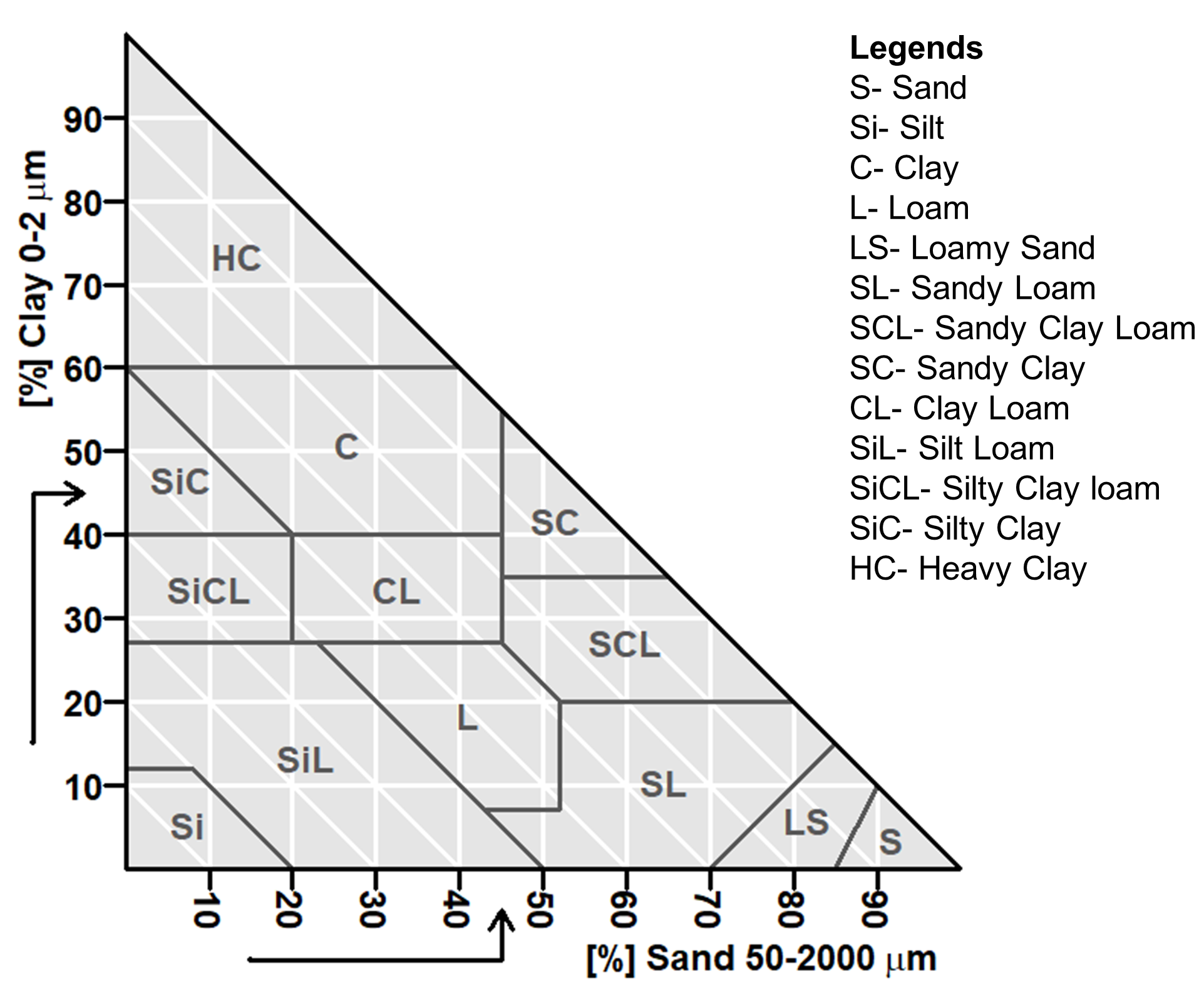
The term soil texture is used to express the relative proportions of the various soil separates in a soil. Qualitatively soil texture represents the feel of the soil materials, while quantitatively soil texture is the relative proportions of the various sizes of particles (i.e., sand, silt, clay) in any soil. Soils are grouped into texture classes based on the relative proportions of sand, silt and clay, and there are 13 such classes in the CSSC (Figure 4.2). The textural class – loam is used to represent soils with about equal proportions of sand, silt, and clay. Generally, a textural class dominated by a single particle size is less suitable for plant growth than a loam. Information on soil textural class is very important as it can guide the soil’s suitability for plant growth and dictate the land use capability, as well as soil management. The movement and retention of water and solutes (e.g., nutrients), as well as heat transfer and aeration, are all affected by soil texture.

In determining the soil textural class using the Canadian soil textural triangle (Figure 4.2), mark the value of sand content on the bottom axis reading from left to right and then take the clay content and mark the value on the vertical axis reading from bottom to the top. Draw a line from the bottom axis identified point parallel to the vertical axis and draw another line from the vertical axis identified point in parallel to the bottom axis. Mark the point where two lines cross and identify the soil textural class. If the point falls on the line of two soil textural classes, the class with finer particles or high clay content will get the designation (customary). Though the third axis presents the silt content, often it is enough to identify textural class with sand and clay data.

Fig_4.2.png — Figure. 4.2. Soil textural triangle following Canadian system of soil classification. The figure is created in R using package ‘soiltexture’. © Asim Biswas is licensed under a CC BY (Attribution) license

Specific surface area of a soil is the total surface area of soil particles per unit mass of soil or per unit volume of soil particles. It is commonly expressed as square meters per gram of soil (mass) or per cubic centimetre (volume) of soil particles. The specific surface area depends on the size as well as shape of the particles. Smaller sized particles contribute to large surface area per unit mass or volume. Similarly, soil particles with flattened or elongated shapes can expose greater surface area per mass or volume than the soil particles of cubic or spherical shape. Clay particles, in addition to their small size, are generally of plate like shape, and they contribute a large surface area per unit mass or volume of soil. While sand particles can have specific surface area of about 1 m² g^-1, clay particles can have specific surface area of as high as several hundred square meters per gram of soil. Specific surface area of any soil material is a fundamental property and is correlated with other important properties such as cation exchange capacity, water retention, nutrient availability, and mechanical properties including plasticity, cohesion and strength.

Soil Structure

Mineral and organic particles in soils are arranged by various forces and at different scales to form distinct structural units called peds or aggregates. Soil structure refers to the arrangement of sand, silt, clay and organic particles into aggregates or peds. These aggregates affect the nature of the system of pores in a soil. Consequently, soil structure has a major influence on water and air movement as well as root growth and the movement of macro- and meso-fauna.

How do Aggregates Form?

Aggregation is the result of several biological, physical and chemical processes across different scales – the atomic or molecular level, the microscopic level, and the macroscopic level or visible scale. Figure 4.3 illustrates aggregate formation across different scales.

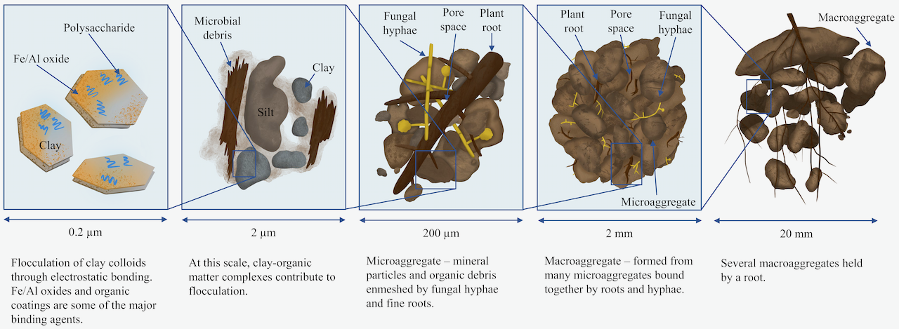
Figure-4.3.-Structure-and-aggregate-formation-2.png — Figure 4.3. Aggregate formation across different scales. Modified from Tisdale and Oades (1982) and adapted from Krzic et al., SoilWeb200 CC-BY. Adapted and modified by Lewis Fausak and licensed under a CC BY (Attribution) license.

At the molecular level, clay particles (with negative charges on their surfaces) attract cations and polar water molecules. Polyvalent cations and water molecules are able to link clay particles by acting as bridges between them. When the soil dries out, the number of water molecules making up these bridges decreases and the clay particles are brought close together. This enables flocculation, which is the first step in aggregate formation.

Organic compounds are also important in forming bridges between clay particles. Long chain molecules (e.g., polysaccharides) are able to come in close contact with the clay, linking them together. Aluminum and iron oxides and hydroxides can perform similar role, creating complex linkages between clay particles, thus, contributing to aggregate formation.

Sand and silt particles carry almost no charge on their surface, but can be linked into micro-aggregates at the microscopic level (≤250 micron) if they have a coating of clay or organic compounds on their surfaces.

At the macroscopic level (≥250 micron), the soil micro-aggregates are bound together into macro-aggregates by fungal hyphae, fine plant roots and other stabilizing agents. It is generally the shape of these macro-aggregates that is described by soil scientists, since they are important for providing the soil with a system of large pores.

A number of factors are recognized as being important for aggregate formation, that all play a role in bringing individual charged clay particles close to each other so that flocculation can occur. These processes include:

wetting and drying cycles
swelling and shrinking of clay particles
freezing and thawing

All of these physical and chemical processes are associated largely with soils that have a high clay content (i.e., in finer textured soils). In sandy soils, aggregate formation is entirely dependent on biological processes, which include:

burrowing activities of earthworms,
production of organic gels by bacteria and fungi that serve as cementing agents and stabilize floccules; for example, hyphae of soil fungi which produce a sticky substance called glomalin that acts as a cementing agent, and
enmeshment of mineral particles by a network of fine roots and fungal hyphae.

The activity of microbes and roots, and the presence of organic matter produces larger aggregates (i.e., macro-aggregates).

Common types of cementing agents in soils are:

organic compounds
clay coatings
Fe/Al oxides
carbonates

Remember that Aggregation = Flocculation + Cementation, where:

Flocculation: is the interaction among soil (clay) particles, when they are brought close together. These interactions include electrostatic and van der Waals forces, and/or hydrogen bonding; and lead to formation of microscopic floccules (or clumps); and

Cementation: is the stabilization of floccules by a cementing agent, such as organic compounds, carbonates, Fe and Al oxides, or clays.

Dispersion of clays

The net negative charge of phyllosilicate particles tend to make them repel each other. When these repulsive forces are strong, particles cannot approach each other and they are said to be dispersed. Mutual repulsion is enhanced by monovalent cations at low concentrations, because under those conditions there is little neutralization of repelling negative charges. Consequently, soil dominated by Na⁺ ions will have clay particles in a dispersed state, more so than a soil where Ca²⁺ or other polyvalent cations are dominant. Dispersion of soil particles is undesirable, since dispersed particles lead to small pores. Water infiltration is thus greatly reduced, leading to standing water at the soil surface.

Types of Aggregates

Soils can either be structureless or aggregated. Single-grained soils are one example of a structureless soil. These soils are dominated by sand particles and there is no aggregate formation. The lack of structure in a sandy soil is due to the fact that sand particles, comprised of primary minerals such as quartz, carry a limited charge. This results in very limited bonding and consequently a very limited flocculation in coarse textured soils.

Massive soils are another example of a structureless soil. These soils have no visible aggregates and are typical of massive clays. When dry, these soils are hard to break apart. The lack of structure in a clay soil can prevent plant growth, as a massive clay lacks sufficient medium and large pores for root development. This type of soil has a very slow rate of water infiltration.

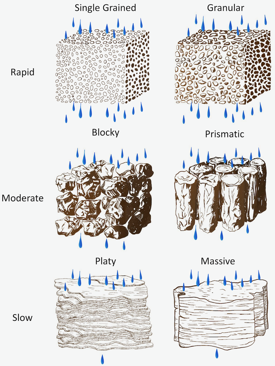
In aggregated soils, soil particles are associated in distinct aggregates or peds. Soil aggregates can be characterized in terms of their: shape (or type), size (fine, medium, or coarse), and distinctness (or strength, such as strong, moderate, or weak). Many types of soil aggregates occur in soils with four principal shapes being spheroidal, platy, block-like (angular blocky with sharp edges and sub-angular blocky with rounded edges), and prism-like (vertically oriented columnar aggregates with rounded tops and prismatic aggregates with flat tops). These structural types (and some sub-types) are illustrated below (Figure 4.4).

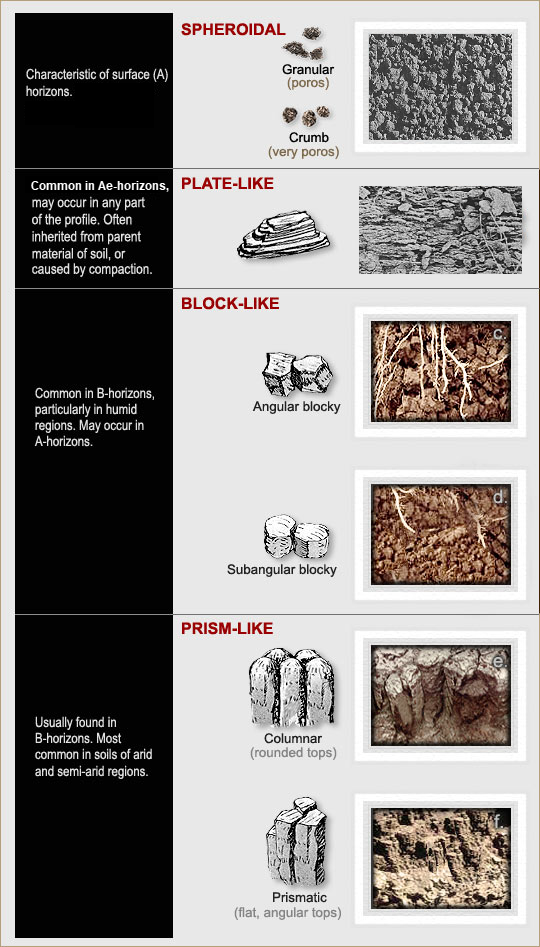
Figure 4.4. Types or shapes of soil aggregates found in mineral soils. Source: © Krzic et al. 2013. SoilWeb200 is licensed under a CC BY-NC-SA (Attribution NonCommercial ShareAlike) license.

Aggregate shape is affected partly by composition and partly by differences in soil development processes. For example, clayey soils often have blocky structure; the columnar structure is frequently associated with sodium clays in semi-arid climates; platy structure often occurs near the soil surface as a result of the freeze-thaw activity.

Soil Structure and Pore Space

Soil structure directly influences the type of pore spaces that exist in a soil. Pores can be classified as: macro-pores (diameter > 0.08 mm) that occur between aggregates or individual grains in coarse-textured soils. Macro-pores readily allow the movement of air, the drainage of water, and provide space for roots and organisms in the soil. Micro-pores (diameter < 0.08 mm) occur within aggregates or between individual clay-size particles. Micro-pores are usually filled with water and are too small to allow much movement of air. Water movement in micro-pores is slow and some of the water tightly held by soil colloids is unavailable to plants.

A well-aggregated clay soil tends to have a balance of large “aeration and drainage” pores, and small “water-retention” pores (Figure 4.5). Good soil structure is associated with small or medium size aggregates with abundant pores both within and between aggregates.

Figure 4.5. Schematic of an A horizon with a porous granular structure, pores between peds or inter-aggregate pores (shown as triangular spaces in the magnifying glass) and within peds or intra-aggregate pores (shown as blue rounded dots). Source: © Krzic et al. 2013. SoilWeb200 is licensed under a CC BY-NC-SA (Attribution NonCommercial ShareAlike) license.

Soil Structure and Water Flow

Soil structure directly influences the size of pores, and through that it impacts other important soil properties such as the rate of water infiltration, water retention, aeration, and drainage (Figure 4.6). Soil with massive structure or platy aggregates can inhibit water flow, while water moves rapidly through pores in soils with granular aggregates and in single grain soils.

Figure-4.6-Structure-and-Drainage.png — Figure 4.6 Water movement as affected by type (shape) of aggregates. Source: USDA 1991. Modified by Lewis Fausak and licensed under a CC BY (Attribution) license.

Impact of Soil Management on Soil Structure

Soil structure is a very important property for water flow and proper aeration in soils. Yet, it is easily subject to deterioration when stresses are applied onto the soil. The stress may be imposed by cultivation, trampling by animals, heavy traffic from logging, dirt bikes and ATVs, etc. Good structure (i.e., balanced macro- and micro-pores) is important for plant growth because it enhances drainage and aeration, while maintaining plant available water within aggregates. If the soil is subject to management practices involving machinery use, it can be vulnerable to compaction (reduction of total pore space by crushing aggregates and infilling of the pore space). Structure can easily deteriorate under the stresses imposed by tractors and farm implements, and even by raindrop impact or foot traffic. Compaction is especially serious when soils are repeatedly subjected to heavy machinery. For this reason, people who manage soils for plant growth respect several soil management principles to maintain good soil structure:

Not running machinery on soil when it is very wet. When water content is very high, the soil cannot offer much resistance to an applied stress. Heavy equipment can easily get stuck in wet soils.
Maintaining an adequate level of calcium or Ca²⁺ content by applying some ground limestone, CaCO₃ to keep the clays flocculated. Calcium is a divalent cation which creates bridges among soil particles, supporting the formation of micro- and macro-aggregates.
Maintaining or adding soil organic matter which can contribute to aggregate strength by binding soil particles together and by encouraging soil microbes which secrete substances that help bind soil particles together.

Repeated tillage, especially under wet conditions, causes the reorientation of particles and compaction of soil just below the depth ploughing. The resulting dense layer of soil, called a “plow pan”, can impede drainage and rooting. Occasional deep cultivation with a “subsoiler” implement, when the soil is dry, may be appropriate to break up such a pan.

Mass-Volume relationships

Mass-volume relationships can be used to define many soil physical properties, including porosity, soil bulk density, and the relative proportions of water and air occupying pore space in a soil.

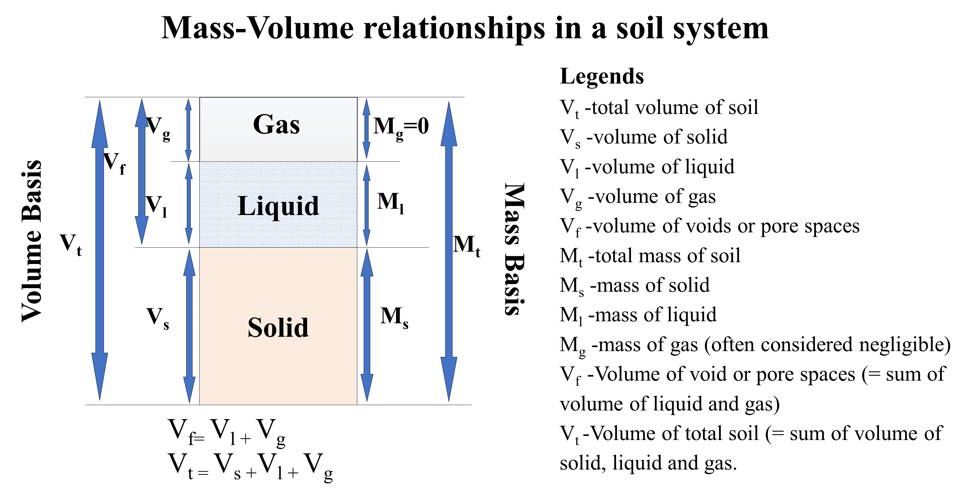
Fig_4.3.png — Figure 4.7. Mass-volume relationships between three phases of a soil system. © Asim Biswas, Univ. of Guelph is licensed under a CC BY (Attribution) license.

The total mass of soil (Figure 4.7) is comprised of the mass of solid (M_s), the mass of liquid (M_l) and the mass of gas (M_g). Note however, that the mass of the gas is negligible, and can be assumed equal to zero.

(1) $\begin{equation*}M_{t} = M_{s} + M_{l} + M_{g}\end{equation*}$

Similarly, the total volume of soil is $V_{t}$ is comprised of the volume of solid ( $V_{s}$ ), the volume of liquid ( $V_{l}$ ), and the volume of gas ( $V_{g}$ ). As the volumes of liquid and gas make up the volume of voids or pores,

(2) $\begin{equation*}V_{f} = V_{l} + V_{g}\end{equation*}$

and the total volume of soil,

(3) $\begin{equation*}V_{t} = V_{s} + V_{l} + V_{g}\end{equation*}$

In the SI system, the unit of mass is kilogram (kg) and the unit of volume is cubic meters (m³). Similarly, in the centimeter-gram-second (CGS) system the unit of mass is gram (g) and the unit of volume is cubic centimeter (cm³).

Densities ( $\rho$ ):

The relationship between mass and volume for any material in a phase is related to its density. The relationship can be written as

(4) $\begin{equation*}Mass = {Volume} \times {Density}\end{equation*}$

(5) $\begin{equation*}Density = \frac{Mass}{Volume}\end{equation*}$

The unit of density is mass unit over volume unit or kg m^-3 (SI unit) or g cm^-3 (CGS unit).

Particle density ( $\rho_{p}$ ): The density of solid (or soil) particles can be calculated as

(6) $\begin{equation*}\rho_{p} = \frac{M_{s}}{V_{s}} = \frac{\text{Mass of solid}}{\text{Volume of solid}}\end{equation*}$

The unit of $\rho_{p}$ is kg m^-3 (SI unit) or g cm^-3 (CGS unit). In calculating $\rho_{p}$ , it is difficult to measure the volume of solids in a soil system; unlike the total volume of soil which includes the volume of air and water. Based on the most common minerals found in soil (i.e., quartz and feldspar), the $\rho_{p}$ of a mineral soil ranges between 2,600 kg m^-3 and 2,700 kg m^-3 (or between 2.6 g cm^-3 and 2.7 g cm^-3). Typically, the average value, 2,650 kg m^-3 (or 2.65 g cm^-3) is used for calculating other soil physical properties. Similarly, $\rho_{p}$ of organic materials is about 1,300 kg m^-3 (or 1.30 g cm^-3).

Liquid or water density ( $\rho_{l}$ ): The density of liquid (or water) can be calculated as

(7) $\begin{equation*}\rho_{l} = \frac{M_{s}}{V_{l}} = \frac{\text{Mass of liquid}}{\text{Volume of liquid}}\end{equation*}$

The unit of $\rho_{l}$ is kg m^-3 (SI unit) or g cm^-3 (CGS unit). For most calculations, the density of water is assumed 1,000 kg m^-3 (or 1.0 g cm^-3).

Dry bulk density ( $\rho_{b}$ ): The dry bulk density can be calculated as

(8) $\begin{equation*}\rho_{b} = \frac{M_{s}}{V_{t}} = \frac{\text{Mass of solid}}{\text{Volume of total soil}}\end{equation*}$

The unit of $\rho_{b}$ is kg m^-3 (SI unit) or g cm^-3 (CGS unit). Note that ρb accounts for only the mass of solid. As the name implies, $\rho_{b}$ includes the mass of dry soil. The $\rho_{b}$ of most mineral soils varies between 1,000 to 1,800 kg m^-3. However, this can be impacted by natural processes (e.g., shrink/swell, aggregation, freeze/thaw) and management practices such as tillage, logging, or grazing. Thus, bulk density is often considered a dynamic property at or near the soil surface, though it is reasonably constant lower in the soil profile. Unlike mineral soils, organic soils (soils with organic matter >30% by weight) generally have ρb ranging between 800 and 1,000 kg m^-3 with values as low as 500 kg m^-3 in soils with very high levels of undecomposed organic matter (e.g., peat soils).

Water content ( $\theta$ )

Water content ( $\theta_{w}$ ) is the amount of water (or liquid) present in a soil system. It can be calculated on a mass basis (known as gravimetric water content, $\theta_{w}$ ) or volume basis (known as volumetric water content, $\theta_{v}$ ), as the ratio of $M_{w}/{M_{t}$ or $V_{w}/{V_{t}$ , respectively. Being a ratio, it is dimensionless. However, the unit of numerator and denominator are often maintained to indicate the type of water content or the calculation procedure. For example, the unit of $\theta_{w}$ is kg kg^-1 or g g^-1 and the unit of $\theta_{v}$ is m³ m^-3 or cm³ cm^-3; thus, the unit indicates the type of water content and the calculation procedure. For example, a value of 0.22 kg kg^-1 of soil indicates the amount of gravimetric water content or $\theta_{w}$ of 0.22. Without an indication of units or specification about the type of water content (gravimetric or volumetric), the value of 0.22 alone can be confusing and misleading. This ratio can further be multiplied by 100 to express the water content in percentage, i.e., 22% water content on a mass or gravimetric basis in this example.

Mass-based or gravimetric water content ( $\theta_{w}$ ): The mass-based water content also known as gravimetric water content can be calculated as,

(9) $\begin{equation*}\theta_{w} = \frac{M_{l}}{M_{s}} = \frac{M_{t} - M_{s}}{M_{s}} = \frac{\text{Mass of liquid (water)}}{\text{Mass of solid}}\end{equation*}$

This is expressed as either dimensionless with specification of gravimetric water content or kg kg^-1 or g g^-1.

Volume-based or volumetric water content ( $\theta_{v}$ ): The volume-based water content also known as volumetric water content can be calculated as,

(10) $\begin{equation*}\theta_{v} = \frac{V_{l}}{V_{t}} = \frac{\text{Volume of liquid (water)}}{\text{Volume of soil}}\end{equation*}$

This is expressed as either dimensionless with specification of volumetric water content or m³ m^-3 or cm³ cm^-3. However, measurement of the volume of liquid in a soil system is very difficult. Thus, often the volumetric water content is estimated from a simple relationship between gravimetric water content and bulk density (see Eq. 14).

Porosity

Porosity is the amount of pore space (or the space occupied by liquid and gas phases) in a soil system. It is an index for the relative volume of pores in the soil. The total volume of pores including that occupied by liquid and gas phases is known as total porosity ( $f$ ). The pores occupied by gas (or air) is known as air-filled (or aeration) porosity and the pores occupied by liquid (or water) is known as water filled porosity. It is the ratio of two volumes (volume of pores to volume of soils) and the units are m³ m^-3 (SI Unit) or cm³ cm^-3 (CGS unit). This ratio can be converted to percentage by multiplying with 100.

Total porosity ( $f$ ): indicates the total pores or voids in a soil system and is calculated as

(11) $\begin{equation*}f = \frac{V_{f}}{V_{t}} = \frac{V_{l} + V_{g}}{V_{t}} = \frac{\text{Volume of voids (liquid + gas)}}{\text{Volume of soil}} = \frac{V_{t} - V_{s}}{V_{t}}\end{equation*}$

The unit of $f$ is m³ m^-3 (SI unit) or cm³ cm^-3 (CGS unit). The ratio can also be converted into percentage by multiplying with 100. In general, for a mineral soil, $f$ varies between 0.3 and 0.6 m³ m^-3. For sandy soils or soils with an abundance of large particle sizes, $f$ tends to be smaller, while for clay dominated soils or soils with finer particles, $f$ tends to be larger. Remember, large size particles can create larger pores than the smaller sized particles. However, the total number of pores and pore volume are higher in soils with finer particles. Note that total porosity does not provide any information about the pore-size distribution. Surface soils tend to have high porosity and the volume of pores generally decrease with depth in the soil profile as the soil bulk density tends to increase.

Water-filled porosity ( $f_{w}$ ): the pores filled with water in a soil system and is calculated as,

(12) $\begin{equation*}f_{w} = \frac{V_{l}}{V_{t}} = \frac{\text{Volume of liquid (water)}}{\text{Volume of soil}} = \theta_{v}\end{equation*}$

The unit of $f_{w}$ is m³ m^-3 (SI unit) or cm³ cm^-3 (CGS unit).

Air-filled porosity or aeration porosity ( $f_{a}$ ): the pores filled with gas (air) in a soil system and is calculated as,

(13) $\begin{equation*}f_{a} = \frac{V_{g}}{V_{t}} = \frac{\text{Volume of gas (air)}}{\text{Volume of soil}}\end{equation*}$

The unit of $f_{a}$ is m³ m^-3 (SI unit) or cm³ cm^-3 (CGS unit). Air-filled porosity is the proportion of the bulk soil occupied by air at any point in time. It is related to the total porosity, and volumetric water content, as both air and water share the same pore volume. Air-filled porosity can then be determined by subtracting the volumetric water content (cm³ of water per cm³ of soil) from the total porosity of the soil. As soil water content varies in time and with soil depth, so does air-filled porosity. Its value will be minimal following significant rainfall or irrigation events. Typically, values should be higher than 0.10 to 0.15 cm³ cm^-3 at field capacity, following drainage.

Relationships among soil physical parameters

While many physical quantities can be calculated from the mass-volume relationships of the three phases, measurement of mass and volumes of different phases are sometimes difficult. Alternatively, easy to measure parameters may be used to estimate parameters that are more difficult to measure. Some useful formulas are provided below.

Relationship between volumetric water content ( $\theta_{v}$ ), gravimetric water content ( $\theta_{w}$ ) and bulk density ( $\rho{b}$ ) can be written as,

(14) $\begin{equation*}\theta_{v} = \theta_{w}\rho_{b}\end{equation*}$

Relationship between total porosity ( $f$ ), bulk density ( $\rho_{b}$ ), and particle density ( $\rho_{p}$ ) can be written as,

(15) $\begin{equation*}f = 1 - \frac{\rho_{b}}{\rho_{p}}\end{equation*}$

Relationship between total porosity ( $f$ ), air-filled porosity ( $f_{a}$ ), and volumetric water content ( $\theta_{v}$ ) can be written as,

(16) $\begin{equation*}f_{a} = f - {\theta_{v}\end{equation*}$

Compaction

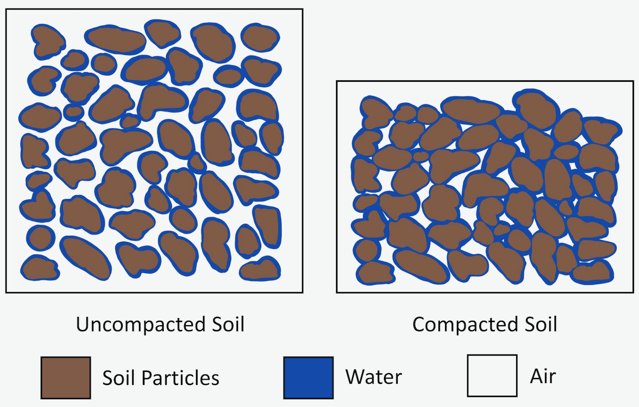
When soil is subjected to pressure, it tends to compress and increase in density. The principal mechanism of soil compression is the reduction of porosity through the partial expulsion of air and/or water from the compressing soil body. For example, static pressure or vibration can cause particles to reorient within the same volume and create a closer packing arrangement. During this reorientation, total porosity, in particular macro-porosity, reduces. In the case of saturated soils, the decrease in porosity takes place as the water is pushed out of macro-pores, unlike in a dry soil where air is pushed out. The expulsion of air is faster than the expulsion of water, which is a slow process as the largest size pores empty first and then the smaller and smaller sized pores. In soils with intermediate soil water content, the air will be expulsed first and then the water. The term compaction is generally applied to the compression of an unsaturated soil body, resulting in a reduction in air volume. While the term consolidation, is generally used for the compression of saturated soil by squeezing out water.

In an agricultural context, a soil is considered to be compacted when the total porosity, in particular the air-filled porosity, is low and restricts aeration, as well as when the soil is so dense and its pores are so small that root penetration and drainage are impeded. Compaction also creates a major issue in field management, particularly tillage. Compaction can occur at the surface (e.g., surface crust) or at the subsurface (e.g., hardpan). A major cause of man-made compaction is related to the use of heavy machinery for agricultural operations. For example, as high as 90% of the field surface can be traversed by tractor wheels during traditional farming operations. Compaction of forest soils is also associated with heavy machinery use, particularly on landings (areas where harvested tress are stored, processed and loaded onto trucks); where it may restrict or prevent the growth of planted tree seedlings or natural regeneration, and where some rehabilitation of compacted areas may be required. Examples of compaction in urban settings include the use of heavy machinery during construction, and excessive trampling by people or bicycles.

Can You Dig It!

What does camping have to do with soils?

Campsite. © Benjamin Hollis is licensed under a CC BY (Attribution) license.

Hiking, mountain biking and tenting can all have significant impacts on the soil. Even by walking, our body weight compresses the soil. Soil compaction reduces the soil porosity and increases soil bulk density. In particular, macro-pores are collapsed, which reduces infiltration and the movement of water through the soil, and can result in overland flow and erosion during rainfall events. The reduction in pore space also reduces aeration, which can negatively affect soil organisms and vegetative growth. Extensive trampling may result in a loss of vegetation, which is commonly seen along hiking trails and at campsites. Campsites typically have a about a 10 m² high-impact area.

Reduction in pore space as a result of compaction. © Lewis Fausak is licensed under a CC BY (Attribution) license.

In high-intensity camping, the impact on soils occurs very quickly, and restoration may take decades. But park rangers and recreation managers are working to create low-impact camping opportunities. In areas where dispersed camping is permitted, tents can be moved daily to reduce the potential for long term impact. Studies suggest that low impact campsites did not compact surface soils to the extent that the root growth of the surrounding vegetation was hindered. But selecting the site to pitch your tent matters; sandy soils are not as susceptible to compaction as fine textured soils. So, avoid sensitive soils and vegetation, stay on the trails, and remember that leave-no-trace camping is more than just packing out your garbage!

References:
Brevik, E.C. and Tibor, M.A. 2014. Impact of camping on soil properties of Strawberry Lake, North Dakota, USA. EGU General Assembly Apr 27-May 2, 2014. Vienna, Austria.

Eagleston, H., and Marion, J.L. 2017. Sustainable campsite management in protected areas: A study of long-term ecological changes on campsites in the boundary waters canoe area wilderness, Minnesota, USA. Journal for Nature Conservation 37: 73-82. doi:10.1016/j.jnc.2017.03.004

Leave No Trace Canada. 2009. Leave no trace principles. https://www.leavenotrace.ca/principle-travel-camp-durable-surfaces

Marion, J.L. and Cole, D.N. 1996. Spatial and temporal variation in soil and vegetation impacts on campsites. Ecological Applications 6(2): 520-530.

WATER RETENTION IN SOILS

Soil can retain water for a substantial amount of time, supporting the growth of plants and soil organisms. Despite the continuous pull from gravity, the water, which enters soil after precipitation or irrigation, stays in the soil for enough time so that plant roots can extract the water to survive. The water is held in the soil in such a way that gases can move through the soil pore spaces and allow oxygen to reach to the roots. Thus, it is critical to understand how soil retains water and acts as reservoir to support life on land. There are two important characteristics of soil water: the amount of water in a given amount of soil (soil water content); and the forces holding water onto the soil matrix (soil water potential). Soil water influences many processes including gas exchange with the atmosphere, the movement of nutrients and chemicals to plant roots, soil temperature, and swelling and shrinking. The forces exerted by the solid matrix on water influences how water is absorbed by plant roots, the drainage that may occur due to gravity, and the extent of upward movement of water and solutes against gravity. These processes are possible because water in soil behaves quite differently than the water in a drinking glass or a swimming pool. Water in soil is strongly associated with the solid particles, particularly soil colloids; and the interactions of water molecules with soil particles changes the behaviour of both.

Properties of water

Soil water influences many processes in soil mainly due to the unique structure of the water molecule. Water is a simple molecular compound, which contains two hydrogen atoms that are covalently bonded to an oxygen atom by sharing electrons in a V-shape. This V-shaped and non-symmetric arrangement of the atoms in the water molecule produces an electric field. The hydrogen atoms, on one side, tend to exhibit electropositive behaviour, while the oxygen atom, on the other side, tends to exhibit electronegative behaviour creating a dipole characteristic. Because of the uneven distribution of electron density, water molecules exhibit polarity and contribute to many properties that allow water to play a unique role in the soil. Water molecules link together as positively charged hydrogen atoms attracts negatively charged oxygen atoms and form a chain-like grouping. Further, due to the polarity of water molecules, they are attracted to charged ions (e.g., Na+, K+, Cl-) and colloidal surfaces (e.g., clay and soil organic matter).

Hydrogen bonding

Because of the polarity of a water molecule, the electronegatively charged oxygen atom can develop an attraction force with the electropositively charged hydrogen as two water molecules come close together. This attraction force creates an intermolecular bond known as hydrogen bond between the protons of the hydrogen atom of one water molecule and the oxygen atom of the other. This force of attraction effectively bonds water molecules together.

Adhesion and cohesion forces

Hydrogen bonds create two forces that are responsible for water retention and movement in soils (Figure 4.8a). The attraction force between water molecules and solid particles is known as adhesion force (force between two different materials). The attraction force between water molecules is known as cohesion force (force between similar materials). Generally, adhesion forces are much stronger than the cohesion forces as water molecules are tightly held onto the soil-solids (also known as adsorption). These tightly bound water molecules further hold onto other water molecules through cohesion forces. Together, the adhesion and cohesion forces make it possible for soil solids to hold water and to allow water movement through the soil. Increasing distance between the water molecule and the solid surface decreases the binding attraction between the water molecule and the solid surface, thus soil water farther away from soil colloids may not be retained onto the surface of a soil particle (e.g., clay).

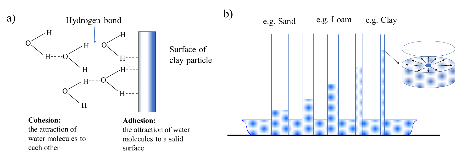
Fig_4.4.png — Figure 4.8. Cohesion and adhesion forces present between water and soil particles (a), and capillary rise of water in different sized (diameter) pores present in different soil textures (b). © Asim Biswas, Univ. of Guelph is licensed under a CC BY (Attribution) license

Capillary rise

If a cylindrical glass tube is kept in contact with a liquid media such as water in a reservoir open to the atmosphere, water will spread over the inside wall of the glass tube. Due to the stronger adhesion force, the attraction between water molecules and the glass wall will be stronger than the cohesion force between the water molecules. Due to this attraction, the glass wall will “pull” water and there will be a rise of water within the glass tube. This is known as capillary rise (Figure 4.8b). The height of capillary rise of water will be determined by the closeness of the glass walls which creates the attraction force and holds the water against the force of gravity. If the walls are close (or the diameter of the tube is small), the adhesion force will be stronger than the cohesion force, and the water will rise higher. On the other hand, if the diameter of the tube is larger, the cohesion force may surpass the adhesion force and the height of rise of water may be small. Consider the situation in soil, where soil pores created by soil particles may be considered as a buddle of tubes. Now, small pores created by small sized particles (e.g., clay) will have a greater height of rise of water compared to the large pores created by the large sized particles (e.g., sand).

Soil water content

Soil water content is the amount of water present in soil. The maximum amount of water a soil can hold is equal to the total volume of pores. When all the pores are filled with water, the soil becomes saturated with water and the water content is known as saturated water content (Figure 4.9). As that saturated soil starts to dry, the amount of water that the soil can hold is determined by various factors including the attraction force between the water and soil particles or the adhesion force. In a saturated condition, all pores are filled with water and the water molecules form layers of water on the soil particles. However, not all the water molecules are equally attracted to the soil particles. Water molecules closest to the soil particle are attracted more strongly than the water molecules far away from the soil particles. Thus, as the distance between soil particles and water molecules increases, the adhesion force between them decreases. Therefore, the water molecules in large sized pores that are farther away from a soil particle surface are weakly held by the soil particles (i.e., the adhesion force is weak). Now, if the saturated soil is allowed to drain freely, the gravitational force surpasses the adhesion force between the soil particles and water molecules. The soil drains until the force created by gravity and the force between soil particles and water molecules equalizes. The amount of water that can be drained by the gravitational force is known as gravitational water (Figure 4.5). The gravitational water leaves a soil system quickly and is not usable by plants or microbes.

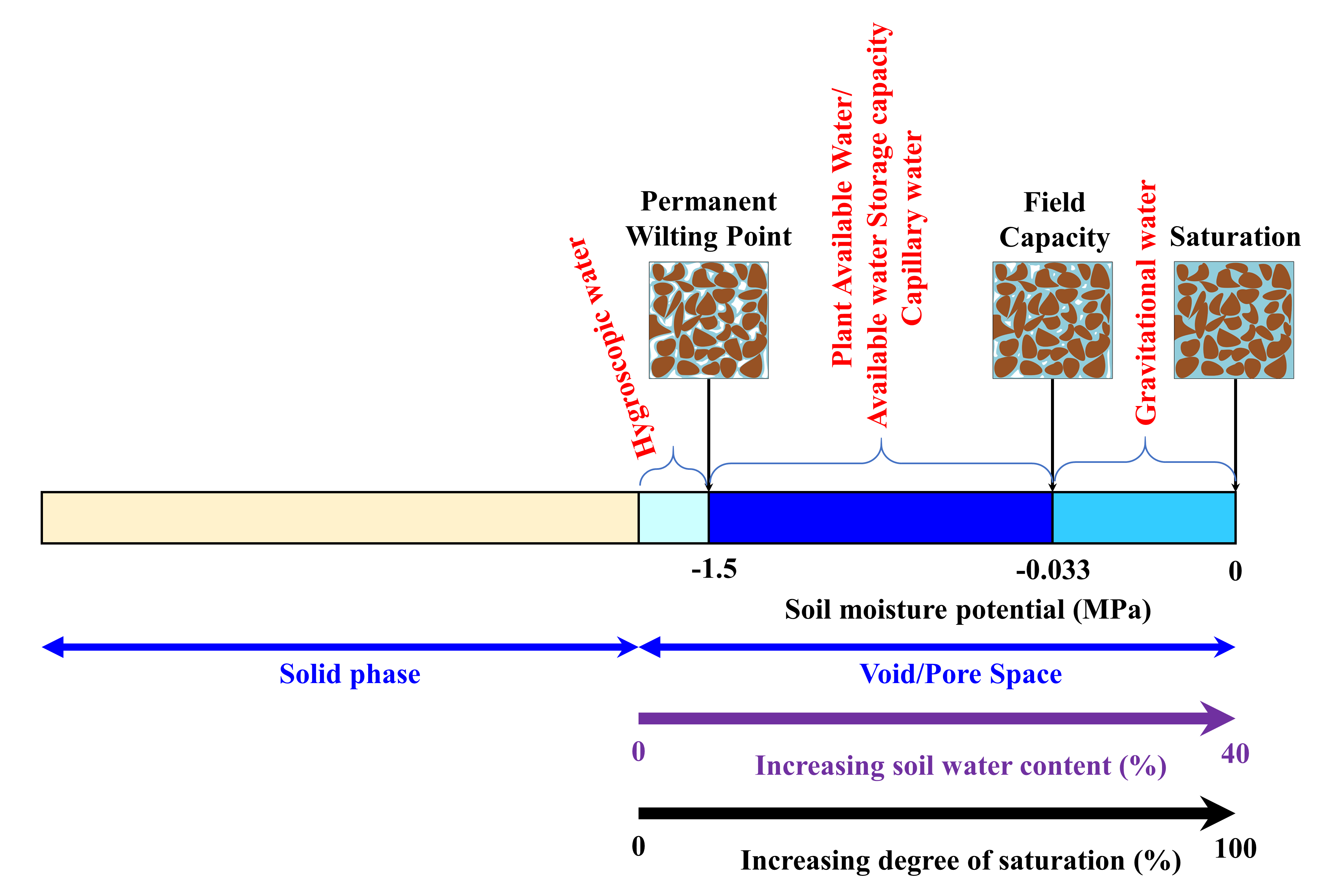
Fig_4.5.png — Figure 4.9. Common terms used to describe soil water content. Adapted from Brady & Weil (2002) and McCauley et al. (2005). Modified by Asim Biswas. CC BY. © Devine and O’Geen (2019) adapted by Asim Biswas, Univ. of Guelph is licensed under a CC BY (Attribution) license.

Once the gravitational water has drained, water is held in soil within the smaller sized (micro- or capillary) pores. Due to their smaller size, the adhesion force between soil particles and water molecules in micro-pores and the cohesion force between the water molecules can hold the water within these pores. External forces, such as the force created by plant roots, can take the water out of these pores. However, as the water molecules closer to the soil solid are attracted by increasing amount of forces, the external force must be stronger than the attraction force to take water out of those pores. Plant roots can only exert pressures up to a certain extent and can uptake a limited amount of water present in soil. The amount of water plants can extract from soil is known as plant available water or available water storage capacity (AWSC). As this water is retained in the capillary pores and held by cohesion forces, it is also known as capillary water (Figure 4.9). Beyond this limit of attraction, the water molecules are attached to the soil particles mainly through adhesion forces. This is known as hygroscopic water. Hygroscopic water generally represents a small amount of the water in soil. This water is not available to plants as plants cannot exert enough force to take hygroscopic water out of the soil. The forces acting between the soil and water molecules can be quantified as soil matric potential, which is described later in this chapter.

As soil starts to dry from a saturated condition, the gravitational water drains out first, followed by plant available water, which decreases as the soil continues to dry out, and eventually may become unavailable as hygroscopic water. The water content when the gravitational water stops, and the plant available water starts is known as field capacity (Figure 4.9). Qualitatively, field capacity is described as the amount of water left in soil two to three days after being saturated (from irrigation or precipitation) and allowed to freely drain by gravitational force. Similarly, the water content at which plants cannot extract any more water from soil is known as permanent wilting point. It is the amount of soil water at which plants cannot take up any more water from soil, start to wilt, and cannot recover (even if water is added subsequently).

Soil water potential

In the previous section, soil water content was defined as the amount (mass or volume) of water in a given mass or volume of bulk soil: gravimetric and volumetric water content, respectively. The measurement of soil wetness is required for understanding the soil water balance, irrigation management, drought assessment and flood forecasting. Soil water also has energy and measurement of the energy of soil water is required to predict the movement of water in soil. Like all mass, soil water moves from locations of relatively high potential to locations of relatively low potential.

What is energy?

Indeed, all mass has energy. The units of energy are Joules (J). Unlike mass, however, energy is difficult to define and conceptualize. An example of the definition of energy from an introductory physics textbook is as follows:

“[energy is a] quantity that is associated with a state (or condition) of one or more objects”

“[energy is] a number that we associate with a system of one or more objects. If a force changes one of the objects by, say, making it move, then the number changes”

These definitions seem a bit “wishy washy”, certainly not as precise as mass (i.e., the amount of matter in an object). The concept of energy becomes clearer when qualified as energy associated with: (1) motion: kinetic energy; (2) separation between an object and an object with known energy: potential energy (gravitational, electrical); and (3) temperature: heat energy.

Soil water potential – units

Because the movement of water in soil is slow (very low velocity), the kinetic energy of soil water is less important than the potential energy of soil water. Hence, soil water energy is simply called soil water potential. Similar to the mass of water in soil that is quantified per unit mass of soil (gravimetric water content) or per unit volume of soil (volumetric water content), soil water potential is also quantified per unit of soil water:

potential energy per unit mass: J kg^-1
potential energy per unit volume: J m^-3 or Pa
potential energy per unit weight: J N^-1 or m (equivalent height of water)

Which units are used to express soil water potential are a matter of choice and it is possible to convert between all three soil water potential units.

Potential energy is always quantified relative to a reference reservoir

Soil water potential is quantified as the difference between the potential energy of soil water and water in a reference reservoir. The reference reservoir used to quantify soil water potential is pure water at atmospheric pressure at a specified elevation.

An example of the reference reservoir would be the surface of water in a beaker sitting on a lab bench. By convention, we set the potential of the reference reservoir equal to zero in order for the potential of the reference reservoir to be the same regardless of its units (i.e., J kg^-1, Pa, or m). Further, this convention allows quick assessment of whether soil water potential is greater than, equal to, or less than the reference reservoir, making it a convenient and intuitive way to quantify and express soil water potential.

Work and formal definition of soil water potential

According to the Soil Science Society of America, the formal definition of soil water potential is: “The amount of work that must be done in order to transport an infinitesimal quantity [mass, volume or weight] of pure water, at a specified elevation and at atmospheric pressure [i.e., the water in the reference reservoir], to the soil water at the point under consideration [without changing its temperature]” (Soil Science Society of America, 1997).

In other words, soil water potential is equal to the amount of work that we must do on water in the reference reservoir to move it to a location in the soil without changing its temperature.

To better understand this definition, the concept of work must be defined. Work has a formal definition in physics, which can be stated as an action on an object that changes the potential energy of the object. For example, by lifting a box from the floor to the top of a table the gravitational potential of the box has increased in proportion to its change in elevation (from floor to table).

So, how much work must be done (i.e., how much effort is required) to transport the water in the reference reservoir to a location in the soils? Analogies to familiar phenomena will help us answer this question. Like soil, sponges have pores and can hold water. Imagine using a dry sponge to clean up some water that has been spilled on a table (or better yet, actually do it). The water on the table is analogous to the water in the reference reservoir and the sponge is analogous to the soil. Without any effort on your part, the water spontaneously moves into the sponge. How much work have you done on the water to transport it into the sponge? Did you break a sweat? No, it did not take any effort at all. In fact, it took less than zero effort, meaning that you did “negative work” on the water (i.e., the sponge did all the work). Now imagine how much effort is required on your part to transport the water from the sponge back to the table surface. You squeeze the sponge to the release the water. Does the sponge release all of the water? No, regardless of how hard you squeeze, the sponge still holds on to a small amount of water. In this case, you did “positive work” on the water in the sponge to transport it back to the table and you still need to do a lot more work to remove the remaining water in the sponge.

Drawing from the analogy of the sponge being the soil and water on the table being the reference reservoir, it can be concluded that the potential of water in the soil is less than the reference reservoir because negative work is required for the soil to absorb water and positive work is required to extract water from the soil. Further, it can be concluded that it is the forces of attraction between soil particles and water molecules that affects the soil water potential. In order to quantify the total potential of soil water, we need to consider all of the forces on soil water affecting its potential and they are summarized in Table 4.2.

Table 4.2. Components of total soil water potential

Forces effecting potential energy	Name of soil water potential component	Reference reservoir	Magnitude of component potential in the reference reservoir
Adsorptive forces between soil particles and water, capillary forces (above the water table; unsaturated soil)	Matric potential, h_m	Water at atmospheric pressure	0
Osmotic forces from dissolved solids	Osmotic potential, h_o	Pure water¹	0
Gravitational forces, elevation	Gravitational potential, h_g	Water at a reference elevation	0
Pressure from overlying water (below the water table; saturated soil)	Pressure potential, h_p	Water at atmospheric pressure	0
All of the above	Total potential, H = h_m + h_o + h_g + h_p	Pure water at atmospheric pressure at a reference elevation	0
¹In pure water the number of dissolved solute particles is zero, and therefore the osmotic potential is zero.

Matric potential is a result of the attraction of water molecules to the soil solids due to adsorption and capillarity (similar to the sponge). As the matric potential reduces the degree of freedom of movement of water relative to the reference reservoir, it is a negative potential. A dry soil has a very low matric potential, while a wet soil has a higher matric potential (i.e., closer to zero).

Osmotic potential is a result of the attraction of water to solutes, which reduce the energy level of water in soil solution. Osmotic potential can impact the uptake of water by plant roots in saline soils, but the solute concentration in most soils is low and does not affect water movement.

Gravitational potential is the result of the pull of gravity, and is defined relative to a specific elevation (e.g., top of the soil profile).

If the soil is completely saturated with water, under a water table for example, then there is no matric potential but a pressure potential resulting from the weight of the overlying water (such as the pressure on your eardrums as you dive at the bottom of a swimming pool).

At any given location in the soil, the total potential of the water is the sum of the soil water potential components, and soil water will flow from locations of high total potential to locations of low total potential. Not every soil water potential component contributes to the total soil water potential in all circumstances. For example, above the water table, the pressure potential is zero because the forces that increase the pressure potential are water pressure forces below the water table. Below the water table, matric potential is zero because the forces that change matric potential, adsorption and capillarity, are very weak in saturated soil.

Soil water retention curve

Soil water has both mass and energy. The amount of soil water (mass or volume) is quantified through measurement of gravimetric or volumetric water content, and soil water potential is quantified relative to reference reservoirs of known potential. Perhaps the next obvious question is whether the amount of soil water (mass or volume) has any relationship to the potential of soil water?

As it turns out, Edgar Buckingham asked the same question back in the late 1800s. He discovered that there was a relationship between the amount of soil water and the soil water potential. He showed that there was a positive relationship between soil water matric potential and soil water content.

Edgar Buckingham was an American soil physicist that understood that mass moves from locations of high total potential to locations of low total potential. It follows that if the total potential of soil water is the same at all locations, there will be zero water flow. Buckingham created a simple soil water system where he was confident that total soil water potential was the same at every location. He placed soil columns of 1.2 m height in a shallow pool of water. Initially the soil in the columns were dry and this caused water from the reservoir to move into the soil, but after a long time, the movement of water from the reservoir into the soil ceased, and the total potential of the soil water was equal at every location in the soil.

Buckingham reasoned that it was the capillary and adsorptive forces that caused water to move from the reservoir into the soil, and that water was held in the soil against the force of gravity – therefore, gravitational and matric potential were the two key components contributing to the total soil water potential. In fact, under the constraint of equal total potential at all locations, gravitational and matric potential must have equal magnitude, but opposite signs. The height to which the water rises in the soil depends on the size of the pores (Figure 4.10a). In soils with smaller pores, the water rise will be higher because of greater capillary forces in small pores. By measuring the water content of the soil at different locations along the soil columns, Buckingham was able to show the relationship between matric potential and soil water content. It is this relationship, between moisture content and the matric potential, which defines the soil water retention curve (Figure 4.10b).

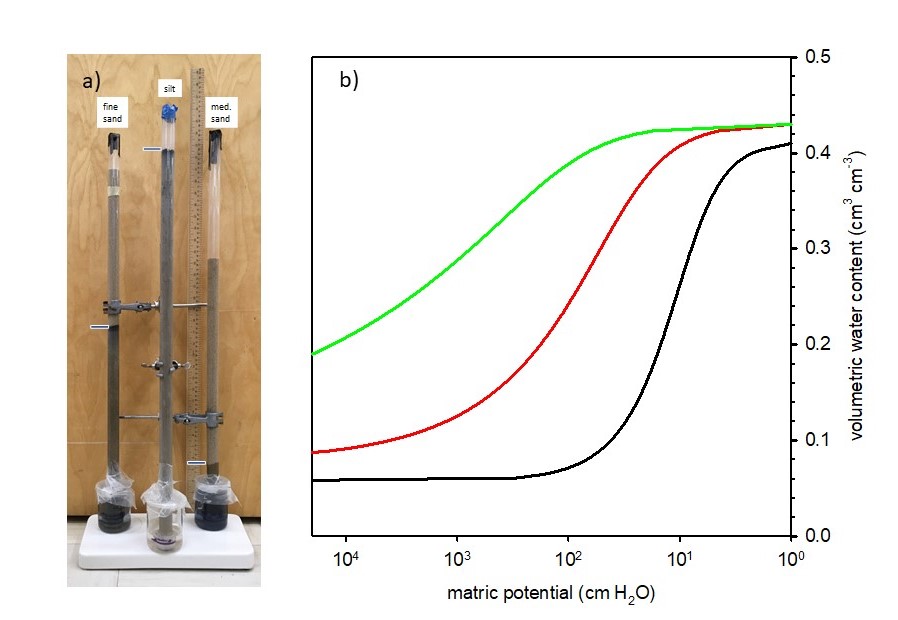
Fig_4.6.jpg — Figure 4.10. Soil water retention simulation of Buckingham’s experiment with columns of fine sand, silt and medium sand (blue lines shown the height to which the water from the reservoir has risen) (a) and soil water retention curves for three soils of contrasting texture (b). © Miles Dyck is licensed under a CC BY (Attribution) license.

Each soil has a unique water retention curve, which can be expressed mathematically as a function: $h_{m}(\theta)$ or $\theta(h_{m})$ (i.e., matric potential is a function of water content and vice versa). To better understand why each soil has a unique water retention curve, soil physicists adopt what is called the capillary tube model of soil pores. This model acknowledges that soil pores behave in a similar way to capillary tubes even though soil pores do have the same shape as capillary tubes. As observed by Buckingham, when a column of dry soil is placed in a water reservoir, water spontaneously rises into the soil just like water rises in a capillary tube placed in a water reservoir. It is the adsorptive and capillary forces (the forces associated with matric potential), that cause the water to rise up into the soil column. Therefore, the height of capillary rise equation can be modified to relate matric potential to the effective radius of water filled pores as follows:

(17) $\begin{equation*}h_{m} \leq \frac{-0.15}{R\ast}\end{equation*}$

where, $h_{m}$ is the matric potential (cm H₂O), and $R\ast$ (cm) is the effective radius of water filled pores.

Therefore, the soil water characteristic curve is a representation of the soil’s cumulative pore-size distribution.

Water availability to plants

Information on how different soils hold and release water is important in understanding water availability for plants and microbes, and forms the basis of water management practices in agriculture, agro-forestry, land reclamation and urban ecosystems. The available water storage capacity (AWSC), provides one approach to assess the proportion of soil water available for plant uptake. Recall that AWSC is defined as the difference in volumetric water content between an upper limit, referred to as field capacity, and a lower limit, referred to as permanent wilting point (Figure 4.9). The available water is calculated for the rooting zone (i.e., m of water per rooting depth). This provides an indication of the amount of irrigation (mm) needed to refill the water reservoir between permanent wilting and field capacity, and answers the two basic questions on when to irrigate and how much water to apply. However, this approach assumes that water is equally available to plants from field capacity down to the permanent wilting point.

Irrigation consists of artificially applying water to maintain its availability to the roots so that plant stress is reduced. Only about two thirds of AWSC is fully available without causing water stress for the plant as at some point, the rate of extraction of water by the plant is faster than the capacity of the soil to supply it (Reicosky and Ritchie, 1976; Rekika et al., 2014). Therefore, not only is maintaining the water supply important, but also the timing at which this water is transferred to the plant though the soil matrix. Better timing can be achieved with irrigation management tools, such as tensiometers and soil-moisture probes, which evaluate water availability within the soil matrix. In the past, overhead and furrow irrigation were extensively used to replenish the soil water reservoir. Currently, drip irrigation and subsurface irrigation are increasingly used, resulting in managing water availability to the plant within a limited soil volume. By adapting irrigation to the specific environmental growing conditions, we can ensure optimal crop productivity and optimal water use (Caron et al., 2015; 2017).

SOIL WATER MOVEMENT

Saturated and unsaturated soil water flow

Water flows in soil from locations of high total potential to locations of low total potential. The magnitude of vertical soil water flow under saturated and unsaturated soil conditions are described by two very similar equations. Flow of water in saturated soils (i.e., when all soil pores are water-filled) is described by Darcy’s Law:

(18) $\begin{equation*}q_{w} = -K_{s}\frac{\Delta H}{\Delta z}\end{equation*}$

where $q_{w}$ is the soil water flux density with units of $\frac{m^3 H_2 O}{m^2 soil\cdot s}$ ; $K_{s}$ is called the saturated hydraulic conductivity having units of $\frac{m^3 H_2 O}{m^2 soil\cdot s}$ per unit of hydraulic gradient; and $\frac{\Delta H}{\Delta z}$ is the hydraulic gradient (i.e., the change in sum of pressure and gravitational potentials over some depth interval, $\Delta z$ ); is dimensionless when $h_{p}$ is expressed in m H₂O.

The negative sign in Darcy’s law is used to specify flow direction. Upward flow (i.e., flow in the increasing z direction, is positive and downward flow, in the decreasing z direction, is negative). Downward flows are associated with positive gradients ( $\frac{\Delta H}{\Delta z}$ > 0), meaning the total potential decreases with decreasing depth.

Edgar Buckingham acknowledged that soils were often unsaturated (i.e., only a fraction of the pores were water-filled), and under these conditions, the hydraulic gradient depends on changes in matric potential within the soil, and that the hydraulic conductivity under unsaturated conditions changes with soil wetness. The result is the Buckingham-Darcy Flux Law:

(19) $\begin{equation*}q_{w} = -K(\theta)\frac{\Delta H}{\Delta z}\end{equation*}$

where, $K(\theta)$ is the hydraulic conductivity as a function of water content, simply referred to as the unsaturated hydraulic conductivity, and $\frac{\Delta H}{\Delta z}$ is the hydraulic gradient (i.e., the change in sum of pressure and gravitational potentials over some depth interval, $\Delta z$ )

Hydraulic Conductivity

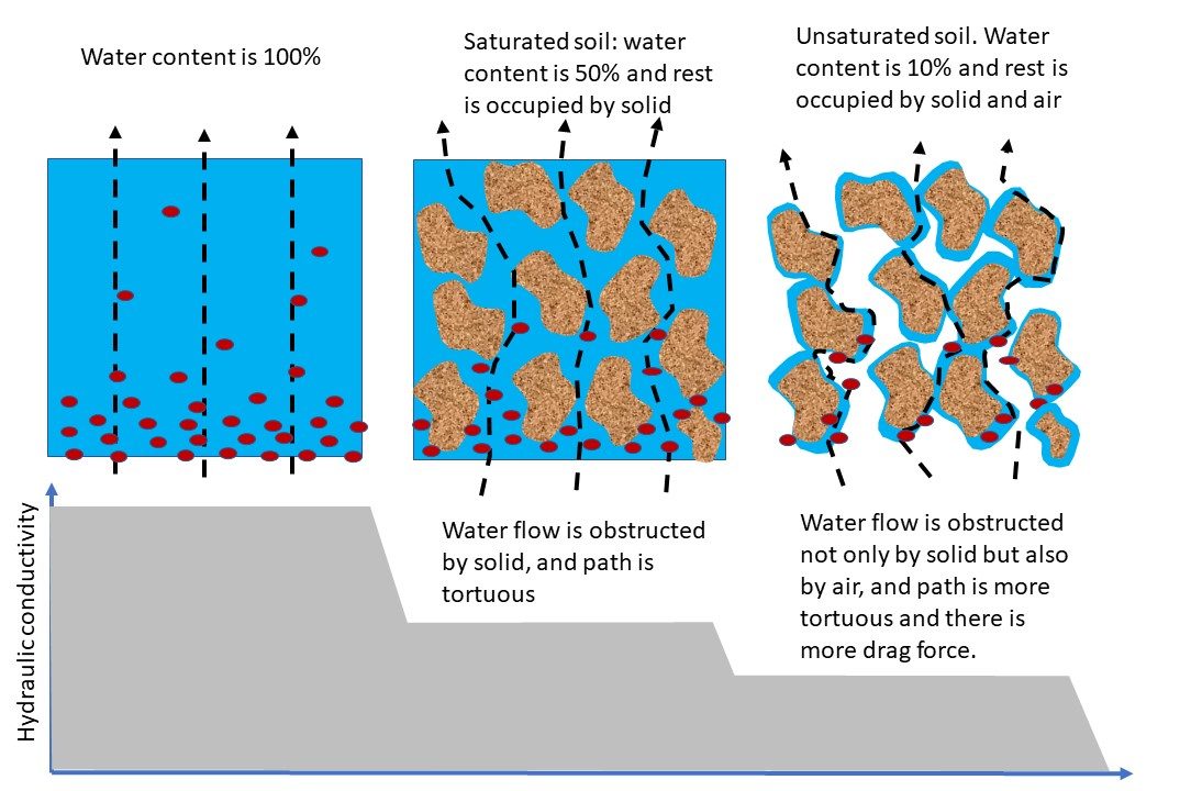
The hydraulic conductivity ( $K$ ) is a soil hydraulic property that represents the soil’s ability to facilitate water flow. Each soil has a unique hydraulic conductivity that is related to the pore-size distribution of the soil. Figure 4.11 shows K as a function of matric potential for soils with three different textures. When saturated, soils with large, continuous pores will have a much greater hydraulic conductivity compared to soils with small, discontinuous pores. As soil water content decreases, the hydraulic conductivity decreases because: (1) the total volume of water-filled pores decreases; and (2) the size of water-filled pores decreases (Figure 4.12). Therefore, soil hydraulic conductivity is a function of the volumetric water content.

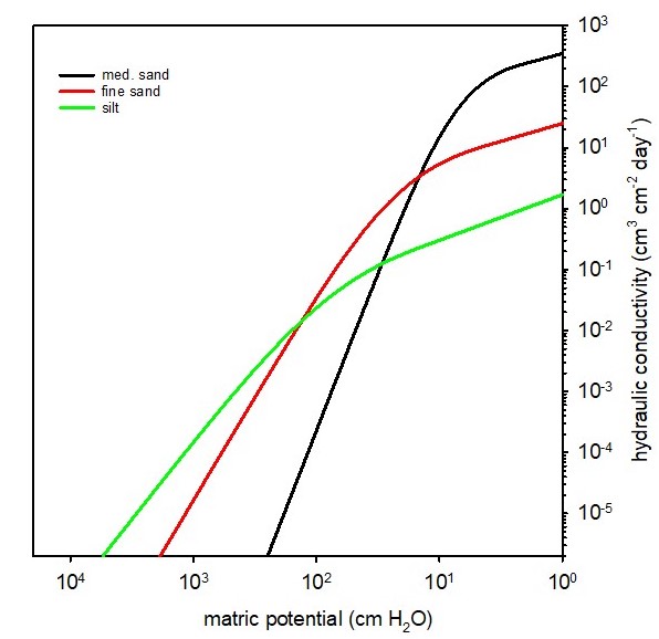
Fig_4.7.jpg — Figure 4.11. Soil hydraulic conductivity curves for three contrasting soil textures. © Miles Dyck is licensed under a CC BY (Attribution) license.

At saturation, the hydraulic conductivity of each soil reaches the maximum value ( $K_{s}$ ), the saturated hydraulic conductivity, but decreases exponentially as the soil becomes drier (y-axis for hydraulic conductivity is on a logarithmic scale). The high Ks of the loamy sand relative to the loam and silty clay loam soils is a reflection of the larger pores associated with coarse-textured soils.

Fig_4.8-e1627251093245.jpg — Figure 4.12. Reduction in flow pathways with decreasing soil water content. © Bing Si is licensed under a CC BY (Attribution) license.

Hydrological processes and the soil water balance

Infiltration and runoff

Infiltration describes the entry of water into the soil through the soil surface, and it determines the surface partitioning of water coming from rainfall or irrigation into either infiltration or runoff (Figure 4.13). The infiltration rate quantifies the volume of water entering a cross-sectional area of soil per unit time (e.g., mm hr^-1). The infiltration rate will generally drop over time due to the gradual saturation of the soil matrix. The infiltration capacity of the soil will depend on both the pore-size distribution and the continuity of the pores, in addition to the antecedent water content. When the rate of supply exceeds the infiltration capacity of the soil at a given time, runoff will occur. Runoff is an important process in water erosion as runoff waters carry and redistribute sediments along slopes, and create rills or gullies at the surface soil.

Figure 4.13. Partitioning of water in the soil. Source: FAO Irrigation and Drainage Paper No. 56 (CC BY-NC-SA). Modified by Jean Caron. © FAO Irrigation and Drainage Paper No. 56 adapted by Jean Caron is licensed under a CC BY-NC-SA (Attribution NonCommercial ShareAlike) license.

Drainage, capillary rise and deep percolation

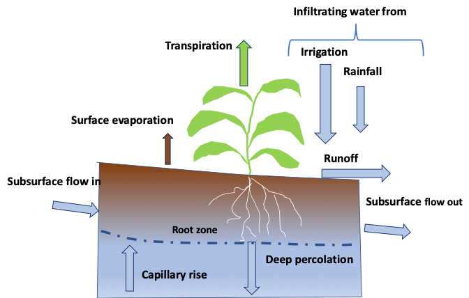
At the bottom of the soil profile, three components interact to affect upward or downward water movement. Percolation refers to the downward movement of water through soil. Drainage is partitioned into two components: surface drainage, which refers to management practices at the land surface to carry excess water towards gullies and ditches; and subsurface drainage which refers to the fraction of water moving downward that is intercepted by a drain tile network, commonly made up of corrugated plastic pipes. Finally, the groundwater component can supply water to the soil through water table fluctuations under saturated conditions or through capillary rise. All three components (percolation, drainage and capillary rise) are time-dependent and therefore have units of volume of water per unit surface area per unit time.

The soil water balance

The soil water budget represents the balance between inputs and outputs from a given soil unit (Eqn. 20). Soil water storage (ΔS) is one component in a water balance. It refers to the change in water storage volume within a given soil unit over a specified time period, and is usually expressed in equivalent height of water per unit time (e.g., mm day^-1).

(20) $\begin{equation*}P + I - ET + Q_i - Q_o - \Delta S - DP = 0\end{equation*}$

where, $P$ = precipitation; $I$ = irrigation; $ET$ = evapotranspiration; $DP$ = drainage and deep percolation; $Q_i$ = other inflow (e.g., capillary rise, and water table fluctuations); and $Q_o$ = other outflow, (e.g., runoff and lateral flow).

Water balance measurements (e.g., using measuring devices called lysimeters) are time and resource consuming, and thus estimates may be made from basic site measurements of soil water content and potential, soil properties and weather data over a given time interval.

SOLUTE TRANSPORT

Fertilizers, pesticides and growth promoters are frequently used in agriculture, and these agrochemicals have greatly contributed to increased crop yields since the 1950s (Ritchie and Roser 2013) . Fertilizers and pesticides are also commonly used in urban settings (e.g., private lawns, city parks) as well as golf courses and playfields. However, excessive application of chemicals and improper management, reduces nutrient use efficiency, enhances greenhouse gas emission and increases the risk of environmental pollution. A prerequisite for optimum application and proper management of chemicals in soil is to understand how chemicals move in soil and toward plant roots.

As described previously, soil is a three-phase system. Chemicals in the form of dissolved constituents (i.e., solutes) can move through soil in the liquid phase. The transport of solutes in soil solution is important for the uptake of nutrients by plant roots. There are two main mechanisms of solute transport in soils: diffusion and mass flow.

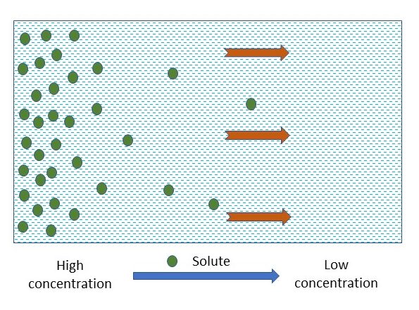
Molecular diffusion

Molecules in a liquid have an internal kinetic energy. As a result, a molecule in a static liquid is in constant motion. The direction in which an individual molecule moves is constantly changing due to its collision with neighboring molecules, known as Brownian motion. While individually, each molecule moves randomly, without a preferred direction, collectively, more ions or molecules tend to move from areas of higher concentration to area of lower concentration (Figure 4.14). In fact, the larger the concentration difference over a certain distance, the faster the spread. To quantitatively measure the rate of the spread we define the flux, as the mass of solute moved perpendicularly across a unit area per unit time (kg m^-2 s^-1), following Fick’s law of diffusion.

(21) $\begin{equation*}q_s = -D_s\frac{\Delta C}{\Delta x}\end{equation*}$

where: $q_s$ is the chemical flux (kg m^-2 s^-1); $\Delta C$ is the concentration difference between two locations ( $\Delta C = C_2 - C_1$ ) separated by distance $\Delta x$ ( $\Delta x = x_2 - x_1$ ); and $D_s$ is and a proportionality constant called the diffusion coefficient (m² s^-1).

Fig_4.10-e1598470337211.jpg — Figure 4.14. Solute (e.g., Cl^–, NO₃^–) flows from high concentration to low concentration in water. © Bing Si is licensed under a CC BY (Attribution) license.

Chemicals are gradually spread out by diffusion with time, and will eventually be uniformly distributed in the media. For a banded fertilizer, fertilizer moves, due to the concentration gradient, from area of high concentration (where the fertilizer band is) to area of low concentration in the surrounding soil. As illustrated by Figure 4.15, the chemicals spread out from the vicinity of the fertilizer band and are distributed horizontally in a bell shape, with the peak at the center of the fertilizer band. With time elapsing, the bell shaped distribution curve extends further away from the fertilizer band, resulting in reduced peak concentration.

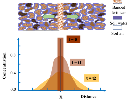
Figure 4.15. Spreading of banded fertilizer with time (t = 0, t₁ and t₂, where t₂ > t₁ > 0) due to diffusion. © Bing Si. CC BY.

In addition to concentration gradients, the diffusion coefficient also determines how fast diffusion occurs and how large the chemical flux is. The volume of water-filled pores for transport, the tortuosity of the transport pathway and drag force all effect the diffusion coefficients in soil.

Mass flow

Solute transport by diffusion occurs within soil solution, but the water as a whole remains stationary. However, when water is under a pressure gradient in the soil, it will move from high potential to low potential, and any constituents in solution or suspension will move with the water. This movement of water and solutes together due to a pressure gradient, is called mass flow. The amount of a solute transported per unit area of soil by mass flow is given by the solute flux ( $q_s$ , kg m^-2 s^-1), which is the product of the water flux and the solute concentration in the solution:

(22) $\begin{equation*}q_s = q_wC\end{equation*}$

where, $q_w$ is the water flux (m s^-1) and $C$ is the solute concentration in water (kg m^-3).

Nutrient transport to roots

Plants develop a network of fine roots for water and nutrient uptake. Through direct contact with soil, roots can intercept nutrients. However, plant roots generally have only direct contact with about 1% of soil volume. Thus, roots need additional mechanisms to access nutrients and water from the remaining 99% of the soil volume.

Mass flow – As a plant transpires water, water is absorbed from soil through the root system. While water flows from the soil in the vicinity of the root hairs, mobile nutrients are carried along with the water, effectively fetching nutrients that are away from the root surface. Mass flow accounts for nutrient uptake of mobile nutrients, such as nitrogen and sulfur. Applying fertilizers in the root zone elevates the nutrient concentration in the solution, enhancing root uptake.

Diffusion – Roots first use up nutrients directly around the root hairs. As the concentration of nutrients around the root system drops, nutrient concentrations may be still high at locations that are slightly farther from the fine roots. This creates a concentration gradient, which moves nutrients from higher concentrated areas toward the surface of roots by diffusion. Note that the chemical flux is proportional to the concentration gradient, consequently the larger the concentration gradient between the root surface and the surrounding soil, the faster the flow of nutrient to the root surface. A large concentration gradient can be created by applying nutrients as close to the root zone and as frequently as possible.

When the transpiration rate is high, mass flow can be dominant mechanism for nutrient uptake. But at low transpiration, nutrient uptake mainly relies on diffusion. When root hairs are not densely distributed in the soil, diffusion from soil to roots can be a bottleneck for root nutrient uptake.

SOIL AERATION AND GAS EXCHANGE

Soil aeration is a critical parameter controlling plant and microbial growth. Accumulation, exchange and consumption of gases all take place in soils. While storage of gases takes place predominantly in large pores, exchange processes are related to gas diffusivity, a property dependent on pore shape, size and connectivity. Accumulation or depletion of a specific gas is controlled by concentration gradients and the presence of sinks and sources of microbial or plant origin. For gases with low solubility in water (e.g., O₂, CO₂), exchange processes take place mainly through the air-filled pores.

As densification of the soil matrix will affect both total porosity and pore-size distribution, poorly structured and compacted soils will experience an important decrease in air-filled porosity, associated with the loss of total porosity and an increase in bulk density. The use of air-filled porosity in characterizing aeration processes is in part related to the ease of measurement and interpretation of the data, but also due to the fact that gas exchange for most soil gases, largely occurs through air-filled pores. As a consequence, air-filled porosity is often used to characterize the potential productivity of the upper soil layer.

Soil air

The composition of the soil air is influenced by the relative ratio of gases (e.g., N₂, O₂, CO₂) in the atmosphere, and by sources and sinks within the soil. Near the soil surface, the soil readily exchanges gases with the atmosphere. However, roots and microorganisms uptake O₂ and produce CO₂ through respiration. As a result, soil air is typically lower in O₂and higher in CO₂. If the gas exchange is restricted (e.g., by wet conditions), anoxic conditions which inhibit plant growth may occur.

Gas diffusion

The main mechanism by which gases move in the soil is through diffusion. Under steady state conditions, a specific gas molecule in the soil air (e.g., O₂ or CO₂) will move according to its concentration gradient following Fick’s first law of diffusion.

Fick’s first law:

(23) $\begin{equation*}J = -D(\frac{dC}{dx})\end{equation*}$

where, $J$ = diffusion flux (g m^-2 s^-1); $D$ = soil gas diffusivity (m² s^-1); and $\frac{dC}{dx}$ = gas concentration gradient (g m^-2)

For example, the diffusive flux of O₂ will be driven by the concentration gradient ( $\frac{dC}{dx}$ ), with the oxygen diffusing from a zone of higher partial pressure (or concentration) in the atmosphere above the soil to a zone of lower partial pressure (concentration) within the soil, as a result of root and microbial respiration (Figure 4.16). For a given concentration gradient, the rate of diffusion is determined the diffusivity ( $D$ ). The diffusivity of oxygen in air is about 10,000 times larger than the diffusivity in water. Thus the oxygen diffusivity of a soil is strongly influenced by pore size, air-filled porosity and the connectivity of air-filled pores.

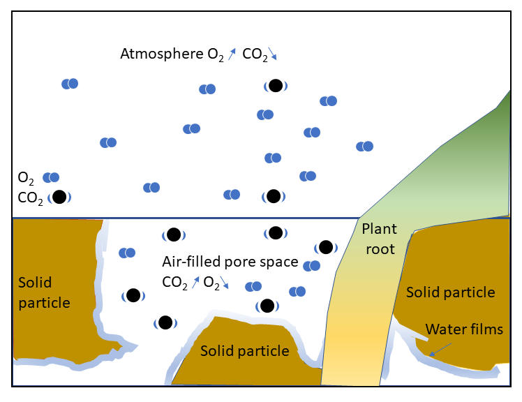
Fig._4.12-e1598452885229.png — Figure 4.16. Diffusion of O₂ and CO₂ driven by concentration gradients of individual gasses near the soil surface. Microbial and root respiration will also lead to a change in local gas concentration as a result of consumption (of O₂) and production (of CO₂). © Jean Caron is licensed under a CC BY (Attribution) license.

The concentration of a gas (e.g., O₂ or CO₂) at depth within the soil depends on both diffusion and biological activity, since organisms both respire and consume gases in the soil. The change of concentration over time associated with oxygen uptake within the soil profile due to root or microbial activity is illustrated in Figures 4.16 and 4.17. The decrease in soil O₂ level at depth is associated with both higher biological activity (i.e., O₂ consumption) and lower diffusivity (i.e., restricted O₂ exchange with the atmosphere). Both biological activity and diffusivity may be affected by land management practices such as irrigation, the addition of organic mater, or compaction due to heavy machinery. As the soil water content increases, gas diffusivity will decrease and therefore the percentage of oxygen will be lower at depth (i.e., moving from blue to green lines in Figure 4.17). Adding compost will increase biological activity, thereby increase O₂ consumption and result in a lower percentage of oxygen at depth (i.e., moving from dashed to solids lines in Figure 4.17). Soil compaction will reduce air-filled porosity, decrease D and result in a decrease in the percentage of oxygen as a function of depth. Gases, such as methane (CH₄), nitrous oxide (N₂O), and ammonia (NH₃), are also exchanged within the soil-plant-atmosphere continuum through similar diffusion and biological transformation mechanisms, and these gases play an important role in climate change.

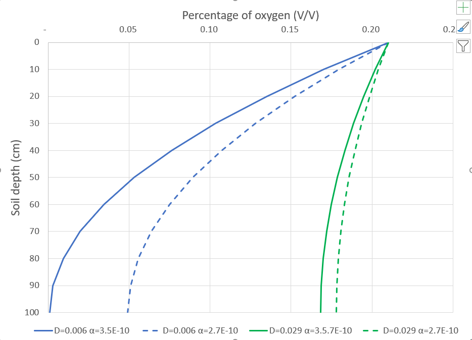
Fig_4.13.png — Figure 4.17. Decrease in soil O₂ levels with depth associated with biological activity (α) and gas diffusivity (D). © Jean Caron is licensed under a CC BY (Attribution) license.

SOIL TEMPERATURE AND HEAT FLOW

Soil temperature is an important property that is essential for many soil processes and reactions that include, but are not limited to, microbial activities, nutrient cycling, root growth and greenhouse gas emissions. Soil temperature also affects seed germination, and therefore is an important consideration for determining seeding date in cold regions such as the Canadian Prairies where winter temperatures drop well below 0°C. For example, the ideal temperature for most crops is around 10°C for seed germination. However, pulses, some peas, lentils and chickpeas, can germinate at around 5°C. Because earlier seeding means a longer growing season, earlier seeding usually means higher yield. Conversely, later seeding can result in later harvesting and greater risk of frost and cold temperatures in the fall, which could greatly reduce crop yield. Therefore, soil temperature is an essential soil property for understanding processes in soil and soil management.

Soil thermal properties are important in determining how quickly a soil heats up in spring, how heat is lost from the soil in winter, and how rapidly the temperature in surface layers change. The heat capacity and thermal conductivity of soils are two important properties, which vary depending on the mineral versus organic content of soils, and with soil water content.

Soil heat capacity: the ability of a substance to hold or store heat. The greater its heat capacity, the more heat it can gain (or lose) per unit rise (or fall) in temperature. Specific heat capacity is the amount of heat (energy) needed to cause a 1°C change in temperature of a unit volume of soil (i.e., the higher the heat capacity, the more energy is needed to cause a small change in temperature). Water has a high heat capacity, while the heat capacity of air is negligible. In soil, as the water content increases, the increase in soil heat capacity is linear (Figure 4.18b). Consequently, a dry soil warms up faster than a wet soil, because the energy required to raise the temperature of a dry soil is lower than that needed for a wet soil. The heat capacity of solid organic matter exceeds that of solid mineral particles, but organic layers are much more porous than mineral soil layers. Thus, the heat storage capacity is lower for organic than mineral soils. Soils with a high heat capacity are resistant to temperature change.

Thermal conductivity: the ability of a soil to conduct heat. Thermal conductivity (λ) describes heat flow in response to a temperature gradient. The thermal conductivity of mineral particles in a soil is about one order of magnitude greater than organic matter; and the thermal conductivity of water is an order of magnitude greater than air (Table 4.3). Organic layers, such as the forest floor, tend to have lower λ than for mineral soils, in large part due to their high porosity and greater air filled porosity. In a mineral soil, thermal conductivity is influenced by soil water content. Since water is a good conductor of heat relative to air, as the water content increases and water films bridge between adjacent solid particles, heat conduction increases quickly (Figure 4.18a). Thus, wet soils conduct heat better than dry soils, while dry soils are good insulators.

Table 4.3. Thermal conductivity (λ) of soil components (modified from de Vries, 1963)

Soil component	λ (J/msK^o)
Quartz	8.368
Clay minerals	2.930
Water	0.594
Organic matter	0.251
Air	0.026

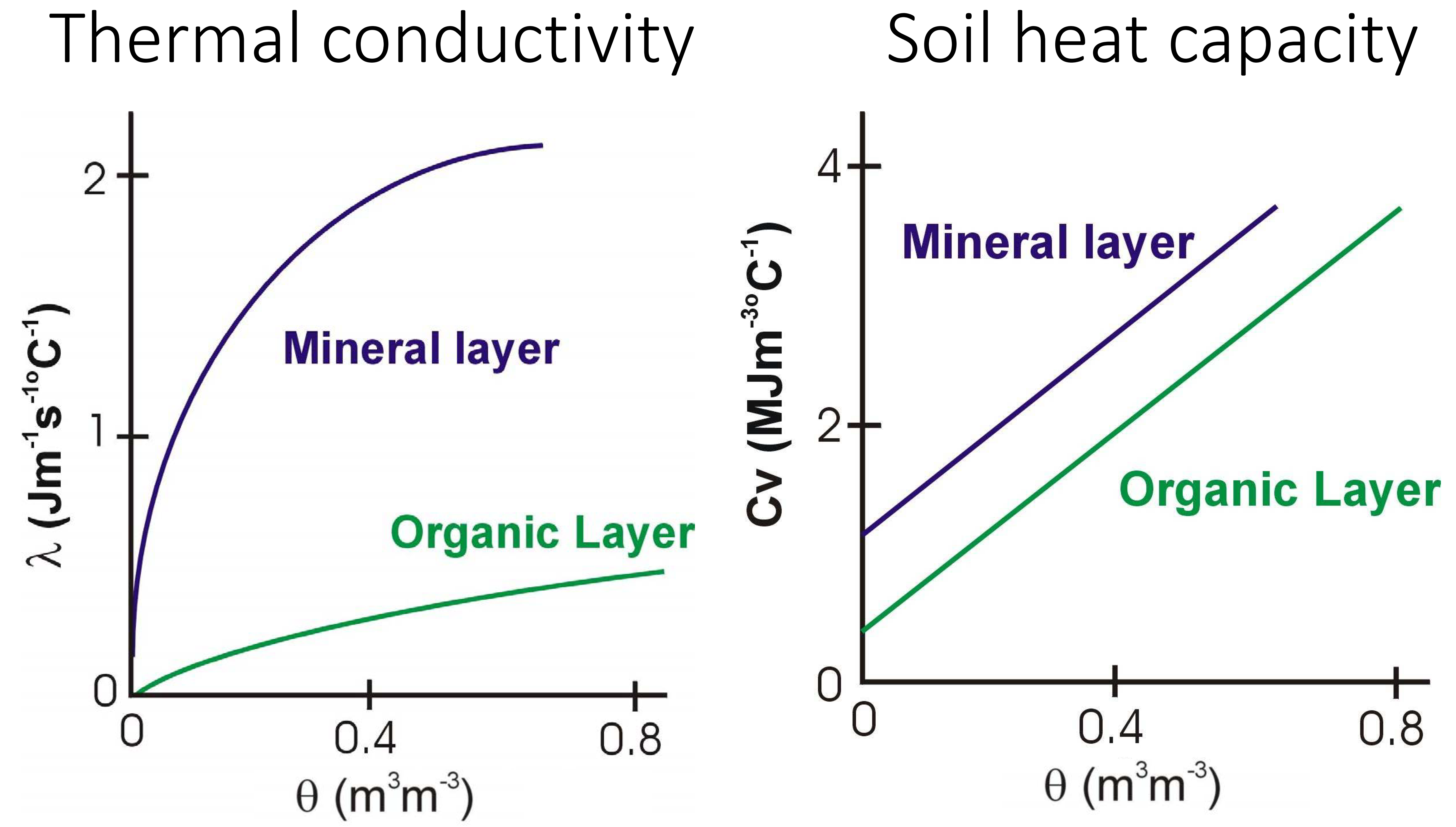
Figure 4.18. Thermal conductivity (a) and soil heat capacity (b) in soil mineral and organic layers. Source: © Krzic et al. 2013. SoilWeb200 is licensed under a CC BY-NC-SA (Attribution NonCommercial ShareAlike) license.

How is soil temperature affected by soil thermal conductivity and heat capacity?

Temperature is a measure of the kinetic energy of individual molecules. It is important for germination and plant growth as well as for activity of soil organisms, and how soil temperature varies over time depends on both climatic factors (e.g., radiation inputs) and soil thermal properties. To give an example, we can compare the surface temperature regimes of two mineral soils with identical texture, SOM, porosity and bulk density, but different soil water content (wet versus dry soil). Initially both soils have the same temperature. On a hot summer day, solar radiation reaching the soil surface is converted to heat energy, which tends to raise the soil surface temperature. The wet soil has a higher thermal conductivity, so it quickly conducts heat downward, away from the surface. Moreover, its high heat capacity means that the surface material would require a large increase in heat content to undergo a temperature increase of 1°C. In contrast, the dry soil cannot conduct heat downward very readily (because of low thermal conductivity), so the surface heat content builds up, and even a small rise in heat content would cause a large rise in temperature (because of the low heat capacity). Thus, the dry soil surface is subjected to extreme temperature fluctuation, and the wet surface is not.

SOIL CONSISTENCY AND STRENGTH

Soil consistence refers to the resistance of soil material to deformation, and the tendency of the soil mass to cohere (stick together) and adhere (stick to other materials). Soil consistence is strongly affected by the clay content and the water content (Figure 4.19). Imagine that we start with dry powdery clay and begin adding water, while we work the sample between our fingers. The shrinkage limit indicates the soil water content where a change in volume occurs (specifically where a loss in soil water no longer results in a reduction in soil volume). At moderately low water content, the soil crumbles, although some pieces stick together. The soil in this condition is said to be “friable“. As we add water, the water content reaches a critical limit or boundary, which is called the plastic limit. The soil suddenly changes in behaviour; it no longer crumbles, but becomes “plastic,” that is, we can deform it and mold it under the stresses applied by our fingers. As we keep adding water to the soil, it remains plastic until another threshold is reached. Suddenly, it is no longer moldable into another shape which it will tend to retain. Instead, the sample has a tendency to flow when stress is suddenly applied. The critical water content at this boundary between plastic and liquid behaviour is called the liquid limit.

These threshold water contents (shrinkage limit, plastic limit and liquid limits) are called Atterberg limits (Figure 4.19). Unlike soil scientists who tend to want to document the resistance of a soil to deformation to preserve the state of a soil for growing trees or crops, engineers want to document how well a soil can resist a stress for building purposes.

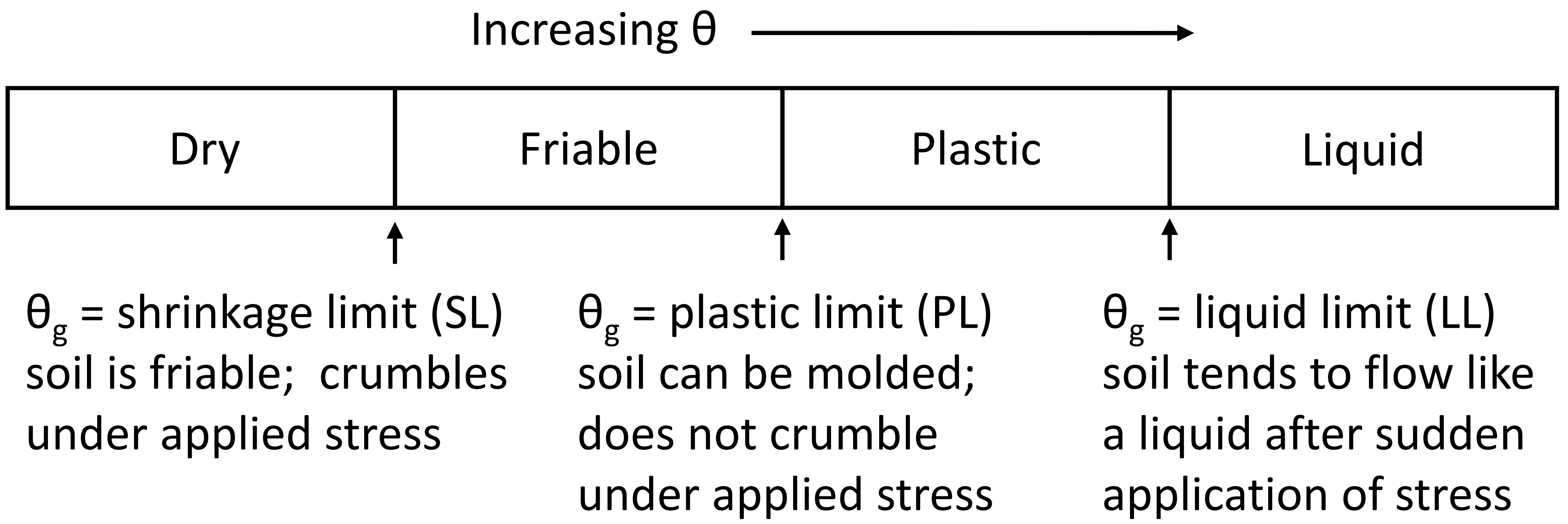
Figure 4.19. Atterberg’s limits. Source: Krzic et al. (2013) SoilWeb200 CC BY-NC-SA. © Krzic et al. 2013. SoilWeb200 is licensed under a CC BY-NC-SA (Attribution NonCommercial ShareAlike) license.

SUMMARY

The soil is a three-phase system: solid, liquid and gas. The magnitude and interaction between the phases determine the behavior and functionality of soil.
Soil texture (i.e., % sand, silt and clay) influences many other soil properties, including water retention, aeration, drainage, and susceptibility to compaction.
Adhesion and cohesion forces are responsible for the retention of water in soils.
Field capacity, permanent wilting point and available water storage capacity (or plant available water) are terms used to describe the water content of a soil for management purposes.
Water movement in soil is driven by differences in soil water potential.
Hydraulic conductivity represents the soil’s ability to facilitate water flow, and is related to the size and connectivity of water-filled pores.
Solutes in soils are transported by diffusion and mass flow.
The main mechanism of gas movement in the soil is through diffusion.
Soil thermal conductivity and heat storage capacity determine how rapidly a soil heats up (or cools down).

STUDY QUESTIONS

Define each of the following terms:
- specific surface area
- fine earth fraction
- soil water potential
Define each of the following terms and identify important distinctions between paired terms:
- soil texture and soil structure
- particle density and bulk density
- field capacity and permanent wilting point
Draw the soil water characteristic curves for a sandy soil and a loam (include axis labels).
Define soil water potential, and explain how the direction of water flows in response to a gradient in total water potential.
List and define the individual forces, which make up total soil water potential.
What is the relationship between matric potential and the size of soil pores?
How might the soil water characteristic curve be used to obtain information about the soil pore-size distribution?
Briefly describe differences in solute transport by mass flow and by diffusion.
How do water-filled pores affect the diffusion of oxygen in soils relative to air-filled pores?
How does compaction by heavy machinery influence oxygen distribution in soils?
In temperature regions (like Vancouver B.C.) where winters are wet and mild, soils may take a long time to warm up in spring. Why do wet soils take a long time to warm up?

WORKED EXAMPLES

Example #1 – bulk density & gravimetric water content

Zineb, a student at the University of British Columbia, collected a soil core from the UBC Farm during summer. The sample is weighed, oven dried at 105ºC for 24 hours (or constant weight) and re-weighed.

Photo by Zineb Bazza, University of British Columbia, Vancouver @ CC BY	The following data were obtained:
	Volume of the core:	330 cm³
	Weight of the metal core:	56.0 g
	Fresh weight of the core + soil	499.4 g
	Oven dry weight of the soil:	386.1 g

Calculate the bulk density and gravimetric water content of this soil sample (show formulas used and units).

Step 1: Calculation of bulk density

We know $\rho_b = \dfrac{M_s}{V_t}$

where $M_s$ = mass of solids and $V_t$ = total soil volume

Thus, $\rho_b = \dfrac{M_s}{V_t} = \dfrac{386.1\,g}{330\,cm^3} = 1.17\,g\,cm^{-3}$

Step 2: Calculation of gravimetric water content

We know that $\theta_w = \dfrac{M_l}{M_s} = \dfrac{M_{fresh} - M_{oven\;dry}}{M_s}$

where

$M_{fresh} = (fresh\,mass\,of\,soil + core) - mass\,of\,core = 499.4\,g -56.0\,g = 443.4\;g$

Thus, $\theta_w = \dfrac{443.4\,g - 386.1\,g}{386.1\,g} = \dfrac{57.3\,g}{386.1\,g} = 0.15\,g\,g^{-1}$

Example #2 – gravimetric & volumetric water content

A soil sample collected from the Chaudière-Appalaches region of Quebec has a gravimetric water content (θ_w) of 0.19 g g^-1 and a bulk density (ρ_b) of 1.26 g cm^-3. What is the volumetric water content (θ_v) of this sample in cm³ cm^-3? Show all formulas, units and full calculation.

We know that $\theta_v = \dfrac{V_l}{V_t}$ and $\theta_w = \dfrac{M_l}{M_s} = \dfrac{M_t - M_s}{M_s}$

Now, $\rho_l = \dfrac{M_l}{V_l}$ or $V_l = \dfrac{M_l}{\rho_l}$ and $\rho_b = \dfrac{M_s}{V_t}$ or $V_t = \dfrac{M_s}{\rho_b}$

Thus, $\theta_v = \dfrac{V_l}{V_t} = \dfrac{\frac{M_l}{\rho_l}}{\frac{M_s}{\rho_b}} = \dfrac{M_l \cdot \rho_b}{M_s \cdot \rho_l} = \theta_w\dfrac{\rho_b}{\rho_l}$

Now, if we consider the density of liquid (or water in this case) = 1 g cm^-3 (in CGS unit), then we can simply write $\theta_v = \theta_w\rho_b$

For the soil sample from the Yukon (showing full units):

$\theta_v = \theta_w\rho_b = 0.19 g g^{-1} \times \dfrac{1.26 \frac{g}{cm^3}}{1 \frac{g}{cm^3}} = 0.24 \frac{cm^3}{cm^3}$

Example #3 – bulk density & porosity

A loam soil in Southern Alberta has a porosity of 48%. What is bulk density of this soil in kg m^-3? Show all formulas you use and the full calculation including units.

Assuming a particle density of $2.65\frac{kg}{m^3}$ and given a porosity of 48% or $0.48\frac{cm^3}{cm^3}$ , the bulk density is $1,378\frac{kg}{m^3}$

This calculation is done by rearranging and solving the following equation:

Porosity $= 1 - \frac{\rho_b}{\rho_s}$ where $\rho_b$ is soil bulk density and $\rho_s$ is soil particle density.

Therefore: $\rho_b = 2.65 \frac{g}{cm^3} - (2.65 \frac{g}{cm^3} \times 0.48) = 1.378 \frac{g}{cm^3} = 1,378 \frac{kg}{m^3}$

Example #4 – Soil water movement

Miles, who teaches introductory soil science at the University of Alberta, took measurements of soil water tension (T) at 3 depths, before and after a large rain event. Unfortunately, some of the measurements were lost.

A) Fill in the two tables below using the following information:

the soil solution contains no salts and the soil is well vented to atmosphere
all three points (or depths) of observation are above the water table (or free water surface)
the reference point is set at the soil surface

[hint: remember that $T = - \text{matric potential}$ ( $h_m$ )]

Table I

Point	Depth in soil (m)	T (m)
A	0	2.3

B	-0.1	2.45

C	-0.25	2.9

Table II

Point	Depth in soil (m)	T (m)
A	0	5.2

B	-0.1	4.4

C	-0.25	4.65

B) Which table belongs to the measurements taken before the rain event, and which after? Briefly explain.

Solution:

determinie $h_g$ : since the reference elevation is at the surface, and the units are m of water, $h_g$ is the same as the depth, i.e., increasingly negative as we move deeper in the soil profile and farther below the reference elevation
recall that the matric potential ( $h_m$ ) = $-\; T$
as the soil solution contains no salts, the osmotic potential $h_o = 0$
as the soil is well vented, and the soil profile is above the water table, $h_p = 0$
recall $h_t = \Sigma(h_g + h_m + h_o + h_p)$
recall that soil water moves from high to low potential, thus you can determine the direction of flow

Table I

Point	Depth in soil (m)	T (m)	h_g (m)	h_m (m)	h_o (m)	h_p (m)	h_t (m)	Direction of flow ( $\downarrow \uparrow$ )
A	0	2.3	0	-2.3	0	0	-2.3
								$\downarrow$
B	-0.1	2.45	-0.1	-2.55	0	0	-2.55
								$\downarrow$
C	-0.25	2.9	-0.25	-3.15	0	0	-3.15

Table II

Point	Depth in soil (m)	T (m)	h_g (m)	h_m (m)	h_o (m)	h_p (m)	h_t (m)	Direction of flow ( $\downarrow \; \uparrow$ )
A	0	2.3	0	-5.2	0	0	-5.2
								$\uparrow$
B	-0.1	2.45	-0.1	-4.4	0	0	-4.5
								$\downarrow$
C	-0.25	2.9	-0.25	-4.65	0	0	-4.9

B) Table I shows the data after the rain, since the direction of water flow in the surface part of the profile (i.e., from point A to B) is downward. Downward water movement implies that water is entering the soil.

Table II shows data before the rain. In Table II, the water is moving upward, from point B to point A, which is an indication that that part of soil profile is drier (probably due to combination of evapotranspiration and water uptake in that part of soil by roots and soil organisms).

Example #5 – Solute transport / nitrate leaching in soil

Fernanda, a student at the University of Saskatchewan conducted a column experiment. The diameter of the soil column was 20 cm. She applied a constant rate of NO₃^– solution on the top of soil column. When the amount of solution collected from the bottom of the column reached steady state (i.e., the flux was constant with time), 30 mL of solution was collected in 30 minutes.

A) Calculate the soil water flux

The water flux is $q_w = \dfrac{V}{At}$ where $A$ is the cross-sectional area of the column ( $\pi r^2$ ); thus,

$q_w = \dfrac{30\,cm^3}{3.14\cdot (10\,cm)^2\cdot 30\,min} = 0.00318\,cm\,min^{-1}$

Fernanda also took a sample of the collected solution and measured the NO₃^–concentration using ion Chromatography (IC). The measured concentration of NO₃^– was 10 μg L^-1.

B) Calculate the NO₃^– flux

The NO₃^– flux can be calculated using Equation # 22:

$q_s = q_wC = 0.00318\,cm\,min^{-1}\,\cdot\,10\,\mu g\,L^{-1}\cdot\,0.001\,L\,cm^{-3}$

$q_s = 3.18\cdot 10^{-5}\,\mu g \,cm^{-2}\,min^{-1}$

Alternatively, we can calculate the flux based on the definition of chemical flux:

$mass\,of\,chemicals = V \cdot C = 30 \,cm^3 \cdot 10 \,\mu g\,L^{-1} \cdot 0.001 \,L \,cm^{-3} = 0.3 \,\mu g$

thus,

$q_s = \dfrac{m}{At} = \dfrac{0.3\, \mu g}{3.14\cdot (10\,cm)^2\cdot 30\,min} = 3.18\cdot 10^{-5}\,\mu g\,cm^{-2}\,min^{-1}$

REFERENCES

Bittman, S., Sheppard, C., and Hunt, D. 2017. Potential for mitigating atmospheric ammonia in Canada. Soil Use and Management 33(2): 263-275. doi:10.1111/sum/12336

Caron, J., Pelletier, V., Kennedy, C. D., Gallichand, J., Gumiere, S., Bonin, S., Bland, B., and Pepin, S. 2017. Guidelines of irrigation and drainage management strategies to enhance cranberry production and optimize water use in North America. Canadian Journal of Soil Science 97(1): 82-91.

Caron, J., Price, J. S., and Rochefort, L. 2015. Physical properties of organic soil: adapting mineral soil concepts to horticultural growing media and Histosol characterization. Vadose Zone Journal 14:1-14.

De Vries, D.A. 1963. Thermal properties of soils. In W.R. van Wijk (ed.) Physics of Plant Environment, John Wiley & Sons, New York. pp. 210-235.

Gregorich, E.G., Turchenek, L.W., Carter M.R., and Angers D.A. 2001. Soil and environmental science dictionary. CRC Press, Boca Raton.

Krzic, M., Wiseman, K., Dampier, L., Grand, S., Wilson, J. and Gaumont-Guay, D. 2013. SoilWeb200: An Online Educational Tool for the APBI 200 course: Introduction to Soil Science. The University of British Columbia, Vancouver [http://soilweb200.landfood.ubc.ca]

Narasimham, T. N. 2007. Central ideas of Buckingham (1907): A century later. Vadose Zone Journal 6(4):687-693. doi:10.2136/vzj2007.0080

Reicosky, D. C., and Ritchie, J. T. 1976. Relative importance of soil resistance and plant resistance in root water absorption. Soil Science Society of America Journal 40(2):293-297.

Rekika, D., Caron, J., Rancourt, G. T., Lafond, J. A., Gumiere, S. J., Jenni, S., and Gosselin, A. 2014. Optimal irrigation for onion and celery production and spinach seed germination in Histosols. Agronomy Journal 106(3):981-994.

Ritchie, H., and Roser M. 2013. Crop Yields. Published online at OurWorldInData.org retrieved from https://ourwolrdindata.org/crop-yields.

Tisdale, J.M. and Oades, J.M. 1982. Organic matter and water-stable aggregates in soils. European Journal of Soil Science 32(2):141-163. doi.org/10.1111/j.1365-2389.1982.tb01755.x

USD-NRCS. 1991. Soil-Water-Plant Relationships. Section 15, Chapter 1, National Engineering Handbook, 2nd edition. https://directives.sc.egov.usda.gov/...tent=18350.wba

About the Authors

Sandra Brown, Assistant Professor Teaching, Faculty of Land and Food Systems, University of British Columbia, Vancouver, BC

Sandra Brown (licensed under a CC-BY-NC-ND license)

Shortly after the 1980 eruption of Mount Saint Helens, I was in the red zone – grey, bleak, ominous, yet beautiful. One year later, that landscape had already begun to transform. I was hooked, I wanted to learn more about this transformation from sediment to soil. Andisols (soils formed in volcanic ash) are my favorite, in part because of their ability to retain water, in part because they are great for growing Colombian coffee!

Asim Biswas, Associate Professor, School of Environmental Science, University of Guelph, Guelph, ON

Asim Biswas (licensed under a CC-BY-NC-ND license)

Growing up on a small subsistence farm in a remote village in India, I recognized soil as the most valuable resource any farm family can have. As I started to play with soils and grow crops with elders, one question always fascinated my young mind, ‘what is there in soils that a small seed can become a big plant or tree?’ My curiosity about soils lead me to study soil science at university. My current research focuses on increasing the productivity and resilience of our food production in an environmentally sustainable way.

Jean Caron, Professor, Soil Science and Agri-Food Engineering, Université Laval, Quebec City, QC

Jean Caron (licensed under a CC-BY-NC-ND license)

At the age of 12, I read an article in Reader’s Digest about Norman Borlaug, a famous agronomist. I made my decision then to become an agronomist and that has never changed. I became interested in the power of math, physics and technology, which lead me to soil physics. As a Professor, I work on water movement in soils, drainage and irrigation management, and soil conservation. Being in the field investigating and solving problems with growers and agricultural engineers is, for me, the most exciting part of my job; having the opportunity to work with passionate farmers and professionals.

Miles Dyck, Associate Professor, Faculty of Agricultural, Life and Environmental Sciences, University of Alberta, Edmonton, AB

Miles Dyck (licensed under a CC-BY-NC-ND license)

I teach courses in soil physics and soil formation/classification. My research focuses on how soil physical processes and properties are affected by human activities. Growing up on a farm in southwestern Saskatchewan, I became curious about how the soils landscapes around my home had developed. In university I learned about soils of Canada and I was hooked! Soils are important for food production, and water and air quality. I am grateful to have the opportunity to make a living by learning about soil.

Bing Si, Professor, College of Agriculture, University of Saskatchewan, Saskatoon, SK

Bing Si (licensed under a CC-BY-NC-ND license)

When I was a teenager, I enjoyed helping out my mom on the farm. But after a long day of harrowing soil using a hoe, I felt the soil was still as hard as a rock. The soil on our farm was clayey and low in organic matter, and when dry, it formed a hard crust. With the question on how to improve the soil, I registered as an agriculture major in university. My current research tries to answer: Why sandy soil can sustain a more water-demanding forest, but not a crop? What is the contribution of deep soil (beyond the 1 m depth) to plant growth?