2.5: What if You Choose the Wrong Variables?
- Page ID
- 4159
\( \newcommand{\vecs}[1]{\overset { \scriptstyle \rightharpoonup} {\mathbf{#1}} } \)
\( \newcommand{\vecd}[1]{\overset{-\!-\!\rightharpoonup}{\vphantom{a}\smash {#1}}} \)
\( \newcommand{\id}{\mathrm{id}}\) \( \newcommand{\Span}{\mathrm{span}}\)
( \newcommand{\kernel}{\mathrm{null}\,}\) \( \newcommand{\range}{\mathrm{range}\,}\)
\( \newcommand{\RealPart}{\mathrm{Re}}\) \( \newcommand{\ImaginaryPart}{\mathrm{Im}}\)
\( \newcommand{\Argument}{\mathrm{Arg}}\) \( \newcommand{\norm}[1]{\| #1 \|}\)
\( \newcommand{\inner}[2]{\langle #1, #2 \rangle}\)
\( \newcommand{\Span}{\mathrm{span}}\)
\( \newcommand{\id}{\mathrm{id}}\)
\( \newcommand{\Span}{\mathrm{span}}\)
\( \newcommand{\kernel}{\mathrm{null}\,}\)
\( \newcommand{\range}{\mathrm{range}\,}\)
\( \newcommand{\RealPart}{\mathrm{Re}}\)
\( \newcommand{\ImaginaryPart}{\mathrm{Im}}\)
\( \newcommand{\Argument}{\mathrm{Arg}}\)
\( \newcommand{\norm}[1]{\| #1 \|}\)
\( \newcommand{\inner}[2]{\langle #1, #2 \rangle}\)
\( \newcommand{\Span}{\mathrm{span}}\) \( \newcommand{\AA}{\unicode[.8,0]{x212B}}\)
\( \newcommand{\vectorA}[1]{\vec{#1}} % arrow\)
\( \newcommand{\vectorAt}[1]{\vec{\text{#1}}} % arrow\)
\( \newcommand{\vectorB}[1]{\overset { \scriptstyle \rightharpoonup} {\mathbf{#1}} } \)
\( \newcommand{\vectorC}[1]{\textbf{#1}} \)
\( \newcommand{\vectorD}[1]{\overrightarrow{#1}} \)
\( \newcommand{\vectorDt}[1]{\overrightarrow{\text{#1}}} \)
\( \newcommand{\vectE}[1]{\overset{-\!-\!\rightharpoonup}{\vphantom{a}\smash{\mathbf {#1}}}} \)
\( \newcommand{\vecs}[1]{\overset { \scriptstyle \rightharpoonup} {\mathbf{#1}} } \)
\( \newcommand{\vecd}[1]{\overset{-\!-\!\rightharpoonup}{\vphantom{a}\smash {#1}}} \)
\(\newcommand{\avec}{\mathbf a}\) \(\newcommand{\bvec}{\mathbf b}\) \(\newcommand{\cvec}{\mathbf c}\) \(\newcommand{\dvec}{\mathbf d}\) \(\newcommand{\dtil}{\widetilde{\mathbf d}}\) \(\newcommand{\evec}{\mathbf e}\) \(\newcommand{\fvec}{\mathbf f}\) \(\newcommand{\nvec}{\mathbf n}\) \(\newcommand{\pvec}{\mathbf p}\) \(\newcommand{\qvec}{\mathbf q}\) \(\newcommand{\svec}{\mathbf s}\) \(\newcommand{\tvec}{\mathbf t}\) \(\newcommand{\uvec}{\mathbf u}\) \(\newcommand{\vvec}{\mathbf v}\) \(\newcommand{\wvec}{\mathbf w}\) \(\newcommand{\xvec}{\mathbf x}\) \(\newcommand{\yvec}{\mathbf y}\) \(\newcommand{\zvec}{\mathbf z}\) \(\newcommand{\rvec}{\mathbf r}\) \(\newcommand{\mvec}{\mathbf m}\) \(\newcommand{\zerovec}{\mathbf 0}\) \(\newcommand{\onevec}{\mathbf 1}\) \(\newcommand{\real}{\mathbb R}\) \(\newcommand{\twovec}[2]{\left[\begin{array}{r}#1 \\ #2 \end{array}\right]}\) \(\newcommand{\ctwovec}[2]{\left[\begin{array}{c}#1 \\ #2 \end{array}\right]}\) \(\newcommand{\threevec}[3]{\left[\begin{array}{r}#1 \\ #2 \\ #3 \end{array}\right]}\) \(\newcommand{\cthreevec}[3]{\left[\begin{array}{c}#1 \\ #2 \\ #3 \end{array}\right]}\) \(\newcommand{\fourvec}[4]{\left[\begin{array}{r}#1 \\ #2 \\ #3 \\ #4 \end{array}\right]}\) \(\newcommand{\cfourvec}[4]{\left[\begin{array}{c}#1 \\ #2 \\ #3 \\ #4 \end{array}\right]}\) \(\newcommand{\fivevec}[5]{\left[\begin{array}{r}#1 \\ #2 \\ #3 \\ #4 \\ #5 \\ \end{array}\right]}\) \(\newcommand{\cfivevec}[5]{\left[\begin{array}{c}#1 \\ #2 \\ #3 \\ #4 \\ #5 \\ \end{array}\right]}\) \(\newcommand{\mattwo}[4]{\left[\begin{array}{rr}#1 \amp #2 \\ #3 \amp #4 \\ \end{array}\right]}\) \(\newcommand{\laspan}[1]{\text{Span}\{#1\}}\) \(\newcommand{\bcal}{\cal B}\) \(\newcommand{\ccal}{\cal C}\) \(\newcommand{\scal}{\cal S}\) \(\newcommand{\wcal}{\cal W}\) \(\newcommand{\ecal}{\cal E}\) \(\newcommand{\coords}[2]{\left\{#1\right\}_{#2}}\) \(\newcommand{\gray}[1]{\color{gray}{#1}}\) \(\newcommand{\lgray}[1]{\color{lightgray}{#1}}\) \(\newcommand{\rank}{\operatorname{rank}}\) \(\newcommand{\row}{\text{Row}}\) \(\newcommand{\col}{\text{Col}}\) \(\renewcommand{\row}{\text{Row}}\) \(\newcommand{\nul}{\text{Nul}}\) \(\newcommand{\var}{\text{Var}}\) \(\newcommand{\corr}{\text{corr}}\) \(\newcommand{\len}[1]{\left|#1\right|}\) \(\newcommand{\bbar}{\overline{\bvec}}\) \(\newcommand{\bhat}{\widehat{\bvec}}\) \(\newcommand{\bperp}{\bvec^\perp}\) \(\newcommand{\xhat}{\widehat{\xvec}}\) \(\newcommand{\vhat}{\widehat{\vvec}}\) \(\newcommand{\uhat}{\widehat{\uvec}}\) \(\newcommand{\what}{\widehat{\wvec}}\) \(\newcommand{\Sighat}{\widehat{\Sigma}}\) \(\newcommand{\lt}{<}\) \(\newcommand{\gt}{>}\) \(\newcommand{\amp}{&}\) \(\definecolor{fillinmathshade}{gray}{0.9}\)Including an Irrelevant Variable
What would be the consequences of including an irrelevant variable in analyzing the dimensional structure of a problem like that of flow past a sphere? Suppose, contrary to fact but just for the sake of discussion, that viscosity is not important in determining \(F_{D}\). Then the functional relationship for \(F_{D}\) would be
\[F_{D}=f(U, D, \rho) \label{contrary} \]
As before, you can start to make this equation dimensionless by forming the same dimensionless drag force \(F_{D} / \rho U^{2} D^{2}\) on the left-hand side. But how about the right-hand side? The three variables \(U\), \(D\), and \(\rho\) cannot be combined to form a dimensionless variable, because there is not enough freedom to adjust exponents to make a product \(U^{a} D^{b} \rho^{c}\) dimensionless; this should be clear from the formal procedure described above for obtaining \(\rho U D / \mu\). Then what takes the place of the Reynolds number on the right side? The answer is that the right side must be a numerical constant: there is no independent dimensionless variable. So if \(\mu\) were not important in flow past a sphere, the dimensionless force \(F_{D} / \rho U^{2} D^{2}\) would be a constant rather than a function of the Reynolds number. To generalize: if one original variable is eliminated from the problem, one dimensionless variable must be eliminated as well. In a graph of \(C_{D}\) vs. \(\mathrm{Re}\) the experimental points would fall along a straight line parallel to the \(\mathrm{Re}\) axis, as shown schematically in Figure \(\PageIndex{1}\). Now look back at the actual graph of \(C_{D}\) vs. \(\mathrm{Re}\) in Figure 2.3.1. Over a wide range of Reynolds numbers from about \(10^{2}\) to greater than \(10^{5}\), \(C_{D}\) is nearly independent of the Reynolds number. Because \(\mu\) is the only variable that appears in the Reynolds number but not in \(C_{D}\), this tells you that \(\mu\) is indeed not important in determining \(F_{D}\) at large \(\mathrm{Re}\). The reasons for this are discussed in Chapter 3.
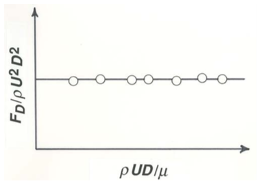
Now you can see why there is some practical advantage to using \(F_{D} / \rho U^{2} D^{2}\) as the dependent dimensionless variable. The other three mentioned above contain \(\mu\), and so in a plot of any one of them against \(\rho U D / \mu\) the segment of the curve for which \(\mu\) is not important would plot as a sloping line rather than as a horizontal line, and the unimportance of \(\mu\) would not be as easy to recognize.
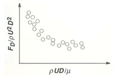
Omitting a Relevant Variable
You should also consider the consequences of omitting an important variable from consideration. For example, if you had not been careful to keep the sphere well away from the wall of the vessel containing the fluid, you would find (Figure \(\PageIndex{2}\)) that the experimental points plot in a scattered band around the curve of \(C_{D}\) vs. \(\mathrm{Re}\) in Figure 2.3.1. This tells you that some other variable is important in determining \(F_{D}\) and that you have inadvertently let it vary—assuming, of course, that your measurements are free of errors in the first place. The obvious culprit is \(y\), the distance of the center of the sphere from the wall (Figure \(\PageIndex{3}\)), because the proximity of the sphere to the solid wall distorts the pattern of flow around the sphere and thus changes the fluid forces on the sphere to some extent. With \(y\) included in the analysis, the functional relationship for \(F_{D}\) is of the form
\[F_{D}=f(U, D, \rho, \mu, y) \label{2.7} \]
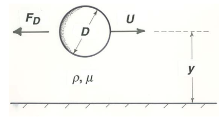
In nondimensionalizing Equation \ref{2.7} you should again expect to have a dimensionless drag force on the left and the Reynolds number on the right. But what happens to the new variable \(y\)? You can use it to form one more independent dimensionless variable, in the same way you formed the Reynolds number. There has to be at least one other such variable, because \(y\) has to appear somewhere on the right side of the nondimensionalized version of Equation \ref{2.7}. A natural choice for this new variable is \(y/D\) (or \(D/y\)). You could instead form another Reynolds number, \(\rho U y / \mu\). But only two of the three variables \(\rho U D / \mu\), \(\rho U y / \mu\), and \( y / D\) are independent of each other: addition of one new independent variable to the problem adds only one new independent dimensionless variable. It is also worth pointing out that you can arrive at the second Reynolds number, \(\rho U y / \mu\), by multiplying the first, \(\rho U D / \mu\), by the new dimensionless variable \( y / D\). This is an illustration of the principle that you can always replace a dimensionless variable in a set of dimensionless variables by another one formed by multiplying or dividing it by one of the others, or with some power or root of one of the others. So in dimensionless form Equation \ref{2.7} is then
\[\frac{F_{D}}{\rho U^{2} D^{2}}=f\left(\frac{\rho U D}{\mu}, \frac{y}{D}\right) \label{2.8} \]
The function in Equation \ref{2.8} would plot as a curved surface in a three-dimensional graph with \(C_{D}\), \(\mathrm{Re}\), and \(y/D\) along the axes (Figure \(\PageIndex{4}\)). The two planes perpendicular to the \(y/D\) axis in Figure \(\PageIndex{4}\) show the range over which \(y/D\) varied in your experiments without your realizing that it is important. The projection of the segment of the surface between these two planes onto the \(C_{D}\)–\(\mathrm{Re}\) plane is the band in which your experimental points would fall. The intersection of the surface with the plane \(y/D = 0\), also shown on the projection, represents the curve you would have gotten if you had always kept the sphere very far away from the wall; it is the same as the curve in Figure 2.3.1.
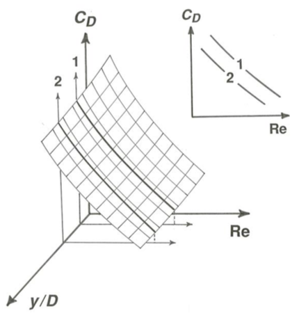
Involving Gravity
You could carry the analysis one step further by moving the sphere horizontally just beneath the free surface of a liquid at rest in a gravitational field (Figure \(\PageIndex{5}\)). Of importance now is not only the distance y of the sphere below the free surface but also the acceleration of gravity \(g\): if the movement of the sphere distorts the free surface, unbalanced gravity forces would tend to flatten the surface again, and surface gravity waves may be generated. Then
\[F_{D}=f(U, D, \rho, \mu, y, g) \label{2.9} \]
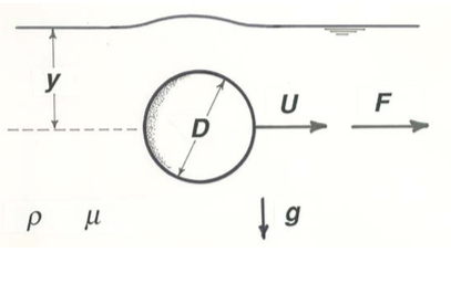
This adds still another independent dimensionless variable, and that variable must include \(g\). There are five possibilities: \(\mu g / \rho U^{3}\), \(\rho^{2} g D^{3} / \mu^{2}\), \(\rho^{2} g y^{3} / \mu^{2}\), \(U^{2} / g D\), and \(U^{2} / g y\), plus obvious variants obtained by inversion and exponentiation. (You could try constructing these by combining \(U\), \(\rho\), \(\mu\), \(D\), and \(y\) three at a time with \(g\) and going through the procedure described above for \(\mathrm{Re}\). You would also get \(y/D\) again in the process.) Any one of these five would suffice to express the effect of \(g\) on the drag force. Again only one is independent, because the others can all be obtained by combining that one (whichever you choose) with either \(\rho U D / \mu\) or \(y/D\). It would be conventional, in a problem like this, to use \(U /(g y)^{1 / 2}\) as the added independent variable. The dimensionless form of Equation \ref{2.9} is then
\[\frac{F D}{\rho U^{2} D^{2}}=f\left(\frac{\rho U D}{\mu}, \frac{U^{2}}{g y}, \frac{y}{D}\right) \label{2.10} \]
The square root of a variable like \(U^{2} / g y\) or \(U^{2} / g D\), with a velocity, a length variable, and \(g\), is called a Froude number, usually denoted by \(\mathrm{Fr}\). It is natural, although not essential, to use \(U^{2} / g y\) here because then each of the four dimensionless variables in the functional relationship can be viewed as being formed by combining \(F_{D}\), \(\mu\), \(y\), and \(g\) in turn with the three variables \(\rho\), \(U\), and \(D\); see the following paragraph for details.
Note
The function in Equation \ref{2.10} would plot as a four-dimensional “surface” in a graph of \(C_{D}\) vs. \(\mathrm{Re}\), \(\mathrm{Fr}\), and \(y/D\). It is difficult to visualize such a graph. A good substitute would be to plot a three-dimensional graph for each of a series of values of one of the independent dimensionless variables. The trouble is that there is an infinite number of these three-dimensional graphs. (I remember once reading somewhere that to express graphically the relationship between two variables you need a page, and to express the relationship among three variables you need a book of pages, and to express the relationship among four variables you need a library of books. For five variables you would need a world of libraries!
Handling Multiple Variables
Suppose that you had realized at the outset that all seven variables in Equation \ref{2.9} are important in the problem. The systematic way of obtaining four dimensionless variables all at once is just an extension of the method described in an earlier section for obtaining the Reynolds number. Form four products by choosing three of the seven variables (the “repeating” variables) to be those raised to the exponents \(a\), \(b\), and \(c\) and using each of the remaining four variables in turn as the one that is raised to the exponent \(1\) (or to any other fixed exponent, for that matter). You can verify for yourself that if you choose \(\rho\), \(U\), and \(D\) as the three repeating variables, the four products \(\rho^{a} U^{b} D^{c} F_{D}\), \(\rho^{a} U^{b} D^{c} \mu\), \(\rho^{a} U^{b} D^{c} y\), and \(\rho^{a} U^{b} D^{c} g\) would produce the four dimensionless variables in Equation \ref{2.10}, except that \(U^{2} / g D\) appears instead of \(U^{2} / g y\). It turns out that for this procedure to work, the constraints on the choice of the three repeating variables are that (1) among them they include all three dimensions \(\mathrm{M}\), \(\mathrm{L}\), \(\mathrm{T}\), and (2) they be dimensionally independent of each other, in the sense that you cannot obtain the dimensions of any one by multiplying together the dimensions of the other two after raising them to some exponents. These constraints just ensure that you get solvable sets of simultaneous equations.


