
5.4: Energy in Open-Channel Flow
- Page ID
- 4179

To address the two channel-transition problems posed earlier, we need to have a closer look at mechanical energy in an open-channel flow, and at how the partitioning of the various components of that mechanical energy, kinetic and potential, are changed at the transition in question.
I noted back in Chapter 3 that the Bernoulli equation is an expression of the work–energy theorem: the work done by the fluid pressure is equal to the change in kinetic energy of the flow. Remember that, in cases like this, if the change in kinetic energy is reversible a quantity called potential energy is defined as minus the work done, and then the sum of kinetic energy and potential energy, often called mechanical energy, is unchanged or conserved. Forces for which this is true, like the fluid pressure in this case, are said to be conservative forces. Gravity is a good example: a ball thrown upward gains potential energy on its way up at the same rate it loses kinetic energy, if the frictional resistance of the air is ignored. Frictional forces, on the other hand, degrade mechanical energy into thermal energy (more commonly called heat or heat energy).
Review the derivation of the Bernoulli equation in Chapter 3 and you will see that fluid pressure is a conservative force: in the absence of friction, the change in pressure potential energy per unit volume between two points \(1\) and \(2\) down a streamline, which is minus the work per unit volume \(- (p_{2} - p_{1})\) by the fluid pressure, is equal to the change in kinetic energy per unit volume, \((\rho/2)({v_{2}}^{2}- {v_{1}}^{2})\), so the two kinds of mechanical energy are interchangeable in this case also. It should therefore seem natural that when the fluid is in a gravity field a term for gravitational potential energy can be included in the Bernoulli equation as well. Because gravitational potential energy is \(mgh\) (where m is the mass of the body under consideration and \(h\) is the elevation relative to an arbitrary horizontal plane), the potential energy per unit volume is \(\rho gh\).
So in the expanded Bernoulli equation the mechanical energy per unit volume of fluid moving along a streamline, \(v^{2} / 2+p+\rho g h\), is constant. This can be written a little more conveniently for our purposes as energy per unit weight of fluid \(E_{w}\). Because weight equals volume multiplied by \(\rho g\),
\[E_{W}=\frac{v^{2}}{2 g}+\frac{p}{\gamma}+h \label{5.3} \]
Note that each term has the dimensions of length; \(E_{w}\) is called the total head, and the terms on the right are called the velocity head, the pressure head, and the elevation head, respectively. In a real fluid, friction degrades mechanical energy to heat as the fluid moves along a streamline. This decrease in mechanical energy from point to point, expressed per unit weight of fluid, is called the head loss. If you add up all three terms on the right in Equation \ref{5.3} the sum decreases downstream, no matter how the values of the individual terms change.
It would be nice to generalize Equation \ref{5.3} so that it applies to an entire open-channel flow, not just to each streamline in it. The problem in doing this is that velocity, elevation, and pressure are not constant from point to point on a cross section. But if there are no strong fluid accelerations normal to the flow direction, pressure is close to being hydrostatically distributed: \(p=\gamma(d-y)\). Then the sum of the elevation head and the pressure head can be written
\(\begin{aligned} h+\frac{p}{\gamma} &=h_{\mathrm{o}}+y+\frac{p}{\gamma} \\ &=h_{\mathrm{o}}+y+\frac{\gamma(d-y)}{\gamma} \end{aligned}\)
\[=h_{\mathrm{o}}+d \label{5.4} \]
where \(h_{\text{o}}\) is the elevation of the channel bottom. Variations in pressure and elevation over the cross section are thus taken into account in Equation \ref{5.3}. Variation in velocity is still a problem, but in turbulent flows the velocity profile is so flat over most of the section that only a small correction need be made in order to replace \(v\) by the cross-sectional mean velocity \(U\). Equation \ref{5.3} can then be written between two cross sections \(1\) and \(2\) in a channel flow that varies only slowly downstream as
\(\text{head loss} =\left(E_{w}\right)_{2}-\left(E_{w}\right)_{1}\)
\[=\frac{U_{2}^{2}}{2 g}+h_{\text{o}2}+d_{2}-\left(\frac{U_{1}^{2}}{2 g}+h_{\text{o}1}+d_{1}\right) \label{5.5} \]
A plot of \(E_{w}\) against downchannel position is called the energy grade line, and the slope of this line (or, generally, curve) is the energy gradient or energy slope.
In a uniform open-channel flow, for which both kinetic energy and potential energy are the same at every cross section but potential energy decreases downstream, the head loss is simply the rate of decrease of elevation head downstream, or in other words the slope of the water surface and bed surface, which is then also equal to the energy slope.
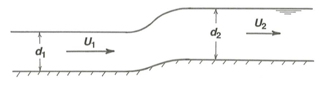
It is often useful to apply Equation \ref{5.5} to an open-channel flow that varies rapidly enough that there is little head loss but slowly enough that the hydrostatic-pressure approximation is not too far wrong. Those conditions are not very restrictive: examples are a gentle rise or fall in the channel bed, as in the first “practical problem” posed earlier in this chapter (Figure 5.2.1) or a gentle expansion or contraction of the channel walls. The development in the rest of this section is meant to address such cases. Equation \ref{5.5} becomes
\[\frac{U_{2}^{2}}{2 g}+h_{\text{o}2}+d_{2}=\frac{U_{1}^{2}}{2 g}+h_{\text{o}1}+d_{1} \label{5.6} \]
A convenient quantity to substitute into Equation \ref{5.6} is \(d+U^{2} / 2 \mathrm{g}\), called the specific head \(H_{\text{o}}\):
\[H_{\mathrm{o}}=d+\frac{U^{2}}{2 g} \label{5.7} \]
Ho, also called the specific energy, is simply the head (i.e., flow energy per unit weight) relative to the channel bottom. Using \(H_{\text{o}}\), Equation \ref{5.6} becomes
\[H_{\mathrm{o} 2}+h_{\mathrm{o} 2}=H_{\mathrm{o} 1}+h_{\mathrm{o} 1} \label{5.8} \]
or
\[H_{\mathrm{o} 2}=H_{\mathrm{o} 1}-\left(h_{\mathrm{o} 2}-h_{\mathrm{o} 1}\right) \label{5.9} \]
Now look at a unit slice parallel to the flow direction in a two- dimensional flow. In other words, you do not have to worry about the sidewalls because they are far away relative to what is happening locally.) Discharge per unit width \(q\) is constant and equal to \(Ud\). Substitution of \(U = q/d\) into the definition for specific head eliminates \(U\) and provides a relation between \(d\) and \(H_{\text{o}}\) for each value of \(q\):
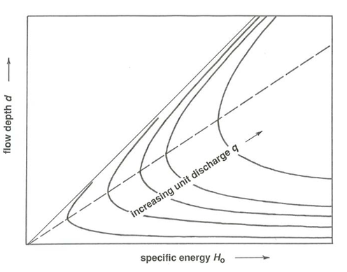
\[H_{\mathrm{o}}=\frac{q^{2}}{2 g d^{2}}+d \label{5.10} \]
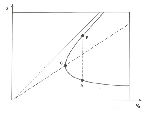
The family of curves of \(H_{\text{o}}\) vs. \(d\) for various values of \(q\) is called the specific-head diagram or specific-energy diagram (Figure \(\PageIndex{1}\)).
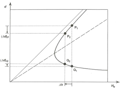
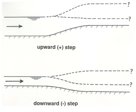
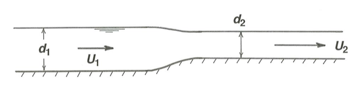
To illustrate the usefulness of the specific-head diagram, suppose that the flow approaching the step shown in Figure 5.2.1 is characterized by values of \(q\), \(d\), and \(H_{\text{o}}\) (i.e.: discharge per unit channel width; depth; and flow energy) that plot at point \(\text{P}_{1}\) in Figure \(\PageIndex{2}\), on the upper part of the curve for the given \(q\). Because the bottom rises by a positive distance \(\delta h = h_{\text{o}2} - h_{\text{o}1}\), by Equation \ref{5.9} the specific head \(H_{\text{o}2}\) associated with the flow downstream of the transition lies a distance \(\delta h\) to the left of \(H_{\text{o}1}\) along the \(H_{\text{o}1}\) axis; \(\text{P}_{2}\) is the corresponding point that represents the flow. Flow depth downstream of the step is therefore smaller by \((\Delta d)_{P}\) in Figure \(\PageIndex{2}\) than in the approaching flow, and by the relation \(q = Ud\) the flow velocity is greater (Figure \(\PageIndex{3}\)). Does that do damage to your intuition?
By virtue of the doubly branched form of the curves in Figure \(\PageIndex{1}\) there can also be an approaching flow, represented by point \(Q_{1}\) on the lower part of the same curve, with exactly the same discharge and flow energy but with shallower depth and higher velocity. In this case the flow downstream of the transition, represented by the point \(Q_{2}\) found by moving a distance \(\delta h\) leftward along the \(H_{\text{o}}\) axis as before, has depth greater by \((\delta d)Q\) than the approaching flow, and smaller velocity (Figure \(\PageIndex{4}\)). Open-channel hydraulicians speak of upper and lower alternate depths.
For points at which the curves of \(d\) vs. \(H_{\text{o}}\) have vertical tangents, depth and velocity do not change in the transition. Flows corresponding to these points are called critical flows. The equation for such points is found in two steps. First, differentiate the function in Equation \ref{5.10} to find \(d H_{\mathrm{o}} / d(d)\), set this derivative equal to zero, and solve for \(q\) as a function of \(d\). The result is
\[q_{c}^{2}=g d_{c}^{3} \label{5.11} \]
where the subscript \(c\) indicates that the equation is for the critical condition of vertical tangency. Then substitute this expression for \(q_{c}^{2}\) into Equation \ref{5.10} to obtain
\[H_{\mathrm{oc}}=\frac{3}{2} d_{c} \label{5.12} \]
again with the subscript \(c\) denoting critical flow.
The locus of points in the specific-head diagram for which the flow is critical is thus a straight line with a slope of \(2/3\). It is shown in Figure \(\PageIndex{1}\) as a dashed line extending upward and to the right from the origin. Flows corresponding to points above the line are subcritical (deeper depths and lower velocities), and flows corresponding to points below the line are supercritical (shallower depths and higher velocities).
Thus, to every combination of discharge per unit width \(q\) and flow energy (represented by \(H_{\text{o}}\)) there correspond two different possible flow states, with different depth and velocity given by the two intersections of the curve of \(d\) vs. \(H_{\text{o}}\) for that \(q\) and the vertical line associated with that \(H_{\text{o}}\). In some kinds of transitions along the channel, the flow is forced all the way from one of these states to the other, thereby passing through the critical state during the transition. Any flow, whatever its origin and therefore whatever its depth and discharge, falls at some point on one of the curves in the specific-head diagram, and is therefore either supercritical or subcritical (or critical). The behavior of that flow in a transition is radically different depending on whether the flow is subcritical or supercritical. This difference in behavior is fundamentally a consequence of the requirement of conservation of flow energy expressed by Equation \ref{5.6}, together with the conservation-of-mass requirement that
\[q=\frac{U_{1}}{d_{1}}=\frac{U_{2}}{d_{2}} \label{5.13} \]
For example, in the transition examined above, the variables \(U_{1}\), \(d_{1}\), \(h_{\text{o}1}\), and \(h_{\text{o}2}\) are all given, and Equations \ref{5.6} and \ref{5.12} then specify exactly which combination of \(U_{2}\) and \(d_{2}\) must hold.
It happens that the condition for critical flow corresponds to a mean-flow Froude number \(U /(g d)^{1 / 2}\) of unity. To verify this, simply substitute Equation \ref{5.11}, the condition for critical flow, into Equation \ref{5.7}, the definition for \(H_{\text{o}}\), to obtain a relation between \(U\) and \(d\) for critical flow: \(U^{2} = gd\), or \(\mathrm{Fr}=1\). Subcritical flows are characterized by Froude numbers less than one, and supercritical flows are characterized by Froude numbers greater than one.
You will see in Chapter 6, on oscillatory flow, that the speed c of a gravity wave in shallow water is \((g d)^{1 / 2}\), where \(d\) is the water depth. If you substitute this wave speed \(c\) for the denominator \((g d)^{1 / 2}\) in the definition of the Froude number, you see that for a Froude number equal to one the mean flow velocity is equal to the speed of surface waves. A water-surface wave that is moving in the upstream direction appears to an observer on the channel bank to be standing still. This means that if the Froude number of the flow is greater than one, wavelike disturbances cannot propagate upstream: the flow coming from upstream cannot know what is in store for it at positions downstream. In subcritical flow, on the other hand, the upstream flow can be influenced, commonly for long distances, by conditions downstream.
That last point is well illustrated by one final consideration of the upward step shown in Figure 5.2.1. As the step height is gradually increased, the corresponding point on the upper branch of the specific head diagram moves leftward and downward from point \(\text{P}\) toward the point of vertical tangent, \(\text{C}\). The farther along the curve the point shifts, the greater is the decrease in flow depth over the step. But there is a limit to this effect: the specific energy cannot decrease beyond that corresponding to the point \(\text{C}\) of vertical tangent, because the flow has to stay on the \(q = \text{constant curve}\). So what happens as the step is raised even further? The flow over the step remains critical and the depth upstream of the step increases. Instead of having no effect on the upstream flow, as was the case for lower steps, the step now acts as a dam: its effect is felt far upstream.
You might be wondering at this point how the flow condition represented by the alternate point on the specific-head diagram can be attained. To see how that might happen, suppose that the geometry of the step in Figure 5.2.1 is changed a bit: after the crest of the step is reached, the channel bottom falls smoothly again to its original height. If now for the approaching subcritical flow with given \(q\) the step height is raised to the point where the flow over the step has just attained the critical condition, represented by point \(\text{C}\) on the curve for the given \(q\) in Figure \(\PageIndex{5}\), the passage of the flow downstream to the original level is manifested on the specific-head diagram as a shift from point \(\text{P}\) to point \(\text{Q}\) vertically below the original point \(\text{P}\) but on the lower (supercritical) limb of the \(q\) curve. The flow is now at the same elevation, and has the same energy (i.e., the same channel-bottom elevation and the same specific head), but it is now flowing at a greatly different combination of depth and velocity, corresponding to supercritical flow (Figure \(\PageIndex{6}\)). What is happening, physically, in contrast to graphically, is that the critical flow at the crest of the step accelerates down the lee side of the step, to attain a supercritical velocity (and, by virtue of conservation of mass, a shallower depth). If the step is raised even beyond what is needed to attain the critical condition, then the flow upstream is dammed, and its depth increases, forcing point \(\text{P}\) upward to the right along the curve for the given \(q\) in the specific-energy diagram.
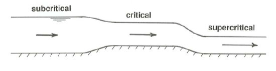
A final comment is that the supercritical flow downstream of the step does not stay supercritical for a very great distance, unless the slope of the bottom downstream of the step becomes much steeper. If the bottom retains its gentle slope, a hydraulic jump is likely to be formed at some point downstream, with the consequence that the flow reverts to its original subcritical condition; see the following section.