7.5: Geostrophic Motion

So far I have discussed some oceanic consequences of the Coriolis effect. Although important, these are on fairly local scales. But the Coriolis effect also plays a striking and fundamentally important role in the dynamics of the large-scale currents and circulations in both the oceans and the atmosphere.

Here is the background you need to know. All of the large-scale motions of the oceans and atmosphere, of the kind you would see on a weather map of North America or a chart of North Atlantic currents, owe their existence to horizontal pressure gradients: changes in pressure from place to place when viewed at the same altitude (in the atmosphere) or the same depth (in the oceans).

This is not the place to describe in much detail how these horizontal pressure gradients come about; I hope it will suffice to say that in the atmosphere they arise from differential heating and cooling and the resulting expansion and contraction of the atmosphere, and in the oceans they arise from a number of effects, including large-scale differences in temperature and salinity and also the horizontal movement and “piling up” of surface waters in response to winds.

Just to give you some feeling for the origin of horizontal pressure differences in the atmosphere, think about a hypothetical convection cell, one that is greatly oversimplified but fundamentally representative of what really happens in the atmosphere on a large scale. Unfortunately this is not something I can expect you to build in your back yard—although essentially the same thing happens in a big tank of differentially heated and cooled water. Figure \(\PageIndex{1}\) shows a gigantic north–south slice through a hypothetical atmosphere. Suppose that, before convection begins, the atmosphere is at the same temperature everywhere at any given altitude. Because air density is a function of temperature, and air pressure is a function of how the air density varies with altitude above the given altitude level, the pressure is the same everywhere at the given altitude, as shown by the horizontal lines in Figure \(\PageIndex{1}\), which represent the intersections of horizontal planes with surfaces of equal pressure (called isobaric surfaces).

Figure \(\PageIndex{1}\): North–south slice through a hypothetical atmosphere, before the action. NP, North Pole; EQ, Equator.

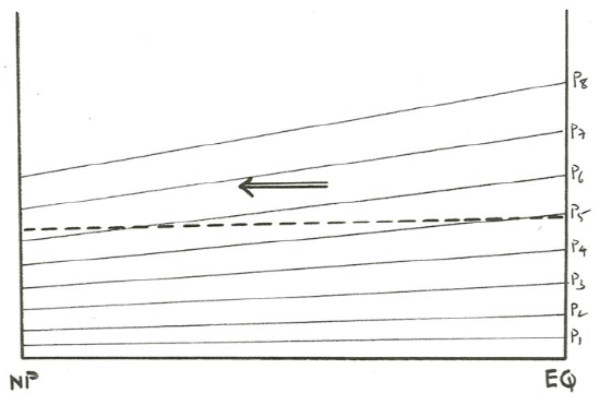
To get the convection cell going, suppose that the atmosphere is heated at low latitudes, near the Equator, and cooled at high latitudes, near the North Pole. At low latitudes the entire column of the atmosphere expands upward, and at high latitudes the entire column of the atmosphere contracts downward, in response to the change in temperature and therefore in density. In response to this expansion and contraction, the isobaric surfaces everywhere above the ground surface take on a poleward slope, as shown in Figure \(\PageIndex{2}\). The effect is a movement of air from low latitudes to high latitudes, as can be seen by considering how the pressure varies across some arbitrary horizontal surface in the atmosphere, shown by the dashed line in Figure \(\PageIndex{2}\). Because of the way the isobaric surfaces cut the horizontal surface, there is a south-to-north decrease in pressure along the horizontal surface, and this pressure gradient causes south-to-north air movement.

Figure \(\PageIndex{2}\): North–south slice through the hypothetical atmosphere, after heating and cooling begins.

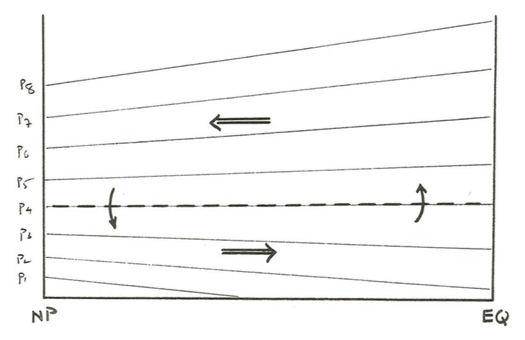
The south-to-north air movement results in a greater total mass of air in an atmospheric column near the North Pole than in an atmospheric column near the Equator. At and near the Earth’s surface, therefore, the atmospheric pressure is greater near the North Pole than near the Equator, so along some horizontal surface low in the atmosphere the horizontal pressure gradient is north-to-south rather than south-to-north. The equilibrium pattern of convective motion then shows (Figure \(\PageIndex{3}\)) northward flow in the upper atmosphere, where the horizontal pressure gradient is to the north, and southward flow in the lower atmosphere, where the pressure gradient is to the south. At some intermediate level, the isobaric surfaces are horizontal, and there is no horizontal motion.

Figure \(\PageIndex{3}\): Circulation produced in the hypothetical atmosphere by heating and cooling.

The foregoing exercise is meant to show how the actual motions in familiar thermal convection cells are qualitatively understandable responses to horizontal pressure gradients set up by differential heating and cooling and consequent expansion and contraction. What I want you to carry away from this example is the idea that there are always going to be horizontal pressure gradients in the atmosphere, which tend to generate winds. (Currents in the deep ocean are generated by such pressure gradients as well.) Now we have to see how the Coriolis acceleration affects these pressure-gradient-generated winds.

I said in an earlier section that the motions of the atmosphere and oceans on the Earth’s surface are dominantly horizontal on a large scale (keep in mind that the slopes of the isobaric surfaces in Figure \(\PageIndex{3}\) are greatly exaggerated) and that only the horizontal component of the Coriolis acceleration has to be considered in these horizontal motions. Think about the fundamental balance of forces that govern these motions. To do a complete job of this we would have to pick apart the governing equations of motion in some detail, but the important effects should make good sense to you without that.

First of all, just as with flow in pipes and channels (Chapter 4), we can think about the balance of forces in the plane parallel to the solid boundary, to which the motions are parallel, and be content in the knowledge that in the normal-to-boundary direction the equation of motion boils down to a balance between the downward weight of the fluid and the upward pressure gradient, as a manifestation of what I called the hydrostatic balance in Chapter 1.

Which horizontal forces need we take into account? The candidates are five: pressure, friction, gravity, Coriolis, and (if the wind blows in a horizontally curved path) centrifugal force. By what was said in the last paragraph, gravity need not be included. And the centrifugal force is really important only in tightly curving winds, as in tornadoes; even around the eye of a hurricane it is not the dominant effect, although it is not negligible either. That leaves pressure, friction, and Coriolis.

I hope it will make sense to you when I claim that, well above the layer of the atmosphere that is in the immediate vicinity of the surface, frictional effects should be very small compared with the other forces. This is indeed the case, as you will see from the outcome of the present line of argument later, but it is not easy to justify. Then the dominant balance of forces is just between the pressure gradient and the Coriolis force. It is this force balance that has such far-reaching consequences for the nature of atmospheric and oceanic motions.

Think about the direction of the wind, relative to the pressure gradient, when the air is moving under the influence of a balance between the pressure- gradient force and the Coriolis force. Use Figure \(\PageIndex{4}\), which is a plan view of some large area over which a horizontal pressure gradient in the atmosphere acts, as a guide. In Figure \(\PageIndex{4}\) the light lines represent the intersections of the isobaric surfaces with a horizontal plane at some fixed altitude at which we are considering the atmospheric motion; these lines, called isobars, are exactly the same as the those they used to show on the weather maps in the newspapers and on television.

Figure \(\PageIndex{4}\): Plan view of a large area of the atmosphere in which there is a horizontal pressure gradient.

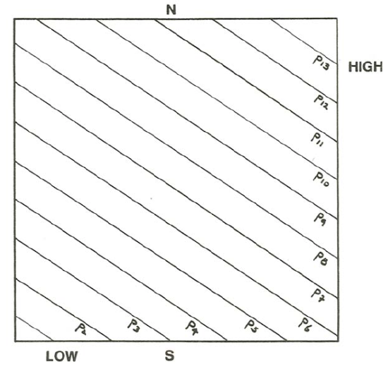
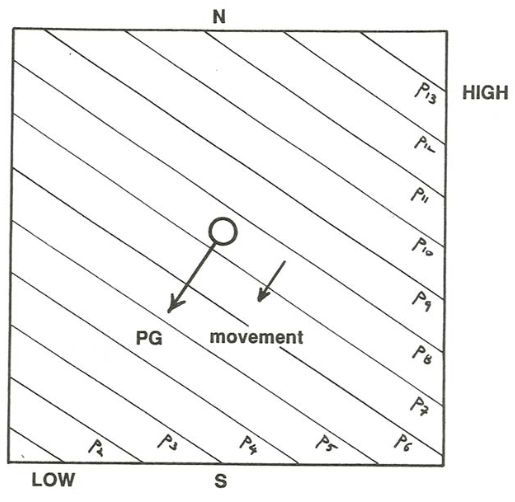
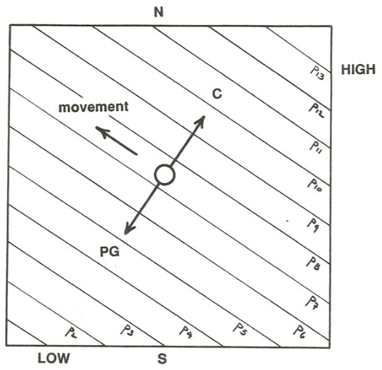
The pressure-gradient force acts at right angles to the isobars, in the direction of decreasing pressure. So (Figure \(\PageIndex{5}\)) in the absence of Coriolis effects the wind should blow straight across the isobars. But on our rotating Earth (Figure \(\PageIndex{6}\)), because the Coriolis force always acts at right angles to the direction of motion, the only way there can be a balance between the pressure gradient and the Coriolis is for the wind to blow along the isobars, not across them!

Figure \(\PageIndex{5}\): In the absence of Coriolis effects, the wind should blow across the isobars toward lower pressure.

Figure \(\PageIndex{6}\): In the presence of Coriolis effects, the wind blows parallel to the isobars.

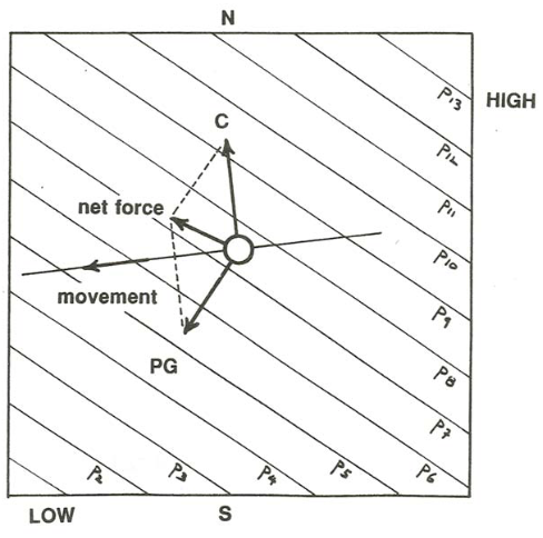
If the startling conclusion in the last paragraph seems fishy to you, or you do not fully understand what is going on, try drawing the balance of the two forces when a parcel of air is moving horizontally in some arbitrary direction other than parallel to the isobars (Figure \(\PageIndex{7}\)). You would see that the resultant of the two forces always has a component off to one side of the assumed direction of motion, and the direction of that component is such as to swing the trajectory of the air lump closer to being along the isobars. There can be no balance until those two force vectors act in directions exactly opposite to each other, and that direction is parallel to the isobars.

Figure \(\PageIndex{7}\): The net force on a parcel of air that is not moving parallel to the isobars is such as to cause its movement to become more nearly parallel to the isobars.

Planetary fluid motion of the kind analyzed above, for which the balance between the pressure-gradient force and the Coriolis force dictates a direction of movement along the isobars, is called geostrophic motion, and the balance of forces itself is called the geostrophic balance. It is of fundamental importance in both the atmosphere and the oceans. In fact, it seems safe to say that geostrophic motion is by far the most striking aspect of large-scale planetary fluid motions.

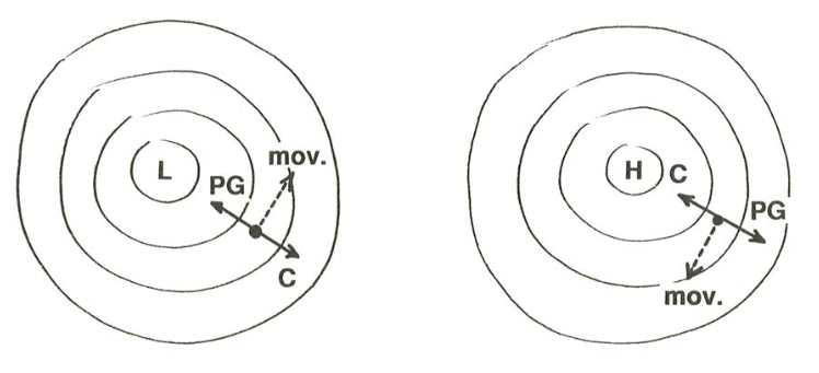
The reality of geostrophic motion is apparent from even a cursory glance at a “real” weather map (one that shows isobars): the winds are almost parallel to the isobars, and in such a sense that in the Northern Hemisphere if you look across the isobars down the pressure gradient, toward the region of low pressure, the wind blows from your left to your right. Another way of saying that is that (in the Northern Hemisphere) the winds move counterclockwise around areas of low pressure and clockwise around regions of high pressure (Figure \(\PageIndex{8}\)).

Figure \(\PageIndex{8}\): In the Northern Hemisphere, winds move counterclockwise around low-pressure area and clockwise around high-pressure areas.