8.2.4: The (S,?)-curve

According to Eq. 8.2.3.2, bulk longshore sediment transport \(S\) is proportional to \(H_{s, b}^{2.5} \sin 2\varphi_b\). The power 2.5 was explained in Intermezzo 8.1 as a sediment load proportional to \(H_{s,b}^2\) transported by a wave-induced longshore current velocity proportional to \(\sqrt{H_{s, b}}\). Both \(H_{s, b}\) and \(\varphi_b\) depend on the offshore wave height, wave period and angle of incidence \(\varphi_0\).

The angle of incidence is relative to the local depth contours, which, in the nearshore zone, are often approximately parallel to the shoreline. Given a relatively constant wave climate along a stretch of coast, alongshore variations in coastline orientation cause gradients in longshore sediment transport and hence cause the coastline orientation to change in time. The relationship between sediment transport \(S\) and angle of wave incidence \(\varphi\) is therefore a central concept in shoreline modelling (see also Sect. 8.3). In order to examine the effect of the angle of incidence on the longshore sediment transport, we consider the situation of straight depth contour lines parallel to the shoreline and compute the sediment transport rate \(S\) from Eq. 8.2.3.7 for a constant offshore wave height and period and for a range of angles of attack (Example 8.2.4.1).

Example \(\PageIndex{1}\)

Input parameters

Offshore wave height: \(H_{rms, 0} = 2\ m\)
Wave period: \(T = 7\ s\)

Required Longshore sediment transport rate \(S\) for different values of \(\varphi_0\)

Method We consider the simple situation of straight depth contour lines parallel to the shoreline. In that case we can use the relation between \(S\) and the deep water wave angle \(\varphi_0\) (Eq. 8.2.3.7). For \(H_0\) we use the deep water wave root-mean-square wave height \(H_{rms, 0}\) and a corresponding value for \(K\) of \(K_{rms} \approx 0.7\). With a value for the porosity \(p = 0.4\) and the relative density \(s = 2.65\), this equation can be written as:

\[S \approx 0.02 c_b H_{rms, 0}^2 \sin 2\varphi_0\label{eq8.2.4.1}\]

We compute \(h_b\) as \(H_{rms, b}/\gamma\) with \(\gamma = 0.8\). This is a rather large value for the breaker index based on \(H_{rms}\), but consistent with the determination of the coefficient value for \(K\).

Figure 8.4: Bulk longshore transport rates \(S\) as a function of the deep water wave angle \(\varphi_0\). The dotted line indicates \(\varphi_0 = 43^{\circ}\). The maximum transport occurs for deep water wave angles somewhat smaller than \(45^{\circ}\) (\(43^{\circ}\) in this case). The angle \(\varphi\) is positive for a transport \(S\) in the direction of a positive alongshore coordinate axis and vice versa.

First choose \(\varphi_0\). Then calculate \(c_b\) using for instance Table A.3 (alternatively, the dispersion relation can be solved using a small computer routine or an explicit approximation). The computation of \(h_b\) requires an iteration (choose \(h_b\), calculate \(H_{rms, b}\) according to Table A.3, check whether \(H_{rms, b}/h_b = \gamma\) if not choose new \(h_b\), repeat process). The sediment transport rate can now be computed using Eq. \(\ref{eq8.2.4.1}\). The results can be found in Table 8.1 and Fig. 8.4.

Table 8.1: Bulk longshore transport rates as a function of the deep water wave angle. In bold: the angle for which the maximum transport is found. Note that \(H_b = \gamma h_b\).

\(\varphi_0 [^{\circ}]\)	\(h_b [m]\)	\(\varphi_b [^{\circ}]\)	\(c_b [m/s]\)	\(S[m^3/s]\)
5	2.72	2.27	4.97	0.069
10	2.71	4.52	4.96	0.136
15	2.69	6.73	4.95	0.198
20	2.66	8.87	4.93	0.253
25	2.63	10.91	4.90	0.300
30	2.59	12.85	4.86	0.337
35	2.54	14.64	4.82	0.362
40	2.48	16.26	4.76	0.375
43	2.43	17.14	4.72	0.377
45	2.40	17.68	4.69	0.376
50	2.31	18.87	4.61	0.364
55	2.21	19.79	4.52	0.340
60	2.09	20.42	4.40	0.305
65	1.95	20.69	4.26	0.261
70	1.79	20.58	4.09	0.210
75	1.59	19.99	3.87	0.155
80	1.35	18.77	3.57	0.098
85	1.01	16.46	3.11	0.043

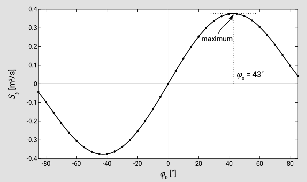
Figure 8.4 shows the longshore sediment transport against the wave angle in deep water. This is a so-called (\(S, \varphi\))-curve; it gives the transport as a function of the wave angle for a given set of wave conditions. The (\(S, \varphi\))-curve indicates that the maximum longshore transport occurs for an angle somewhat smaller than \(\varphi_0 = 45^{\circ}\). The term \(\sin (2\varphi_0)\) in Eq. 8.2.3.7 would suggest a maximum of \(S\) at exactly \(\varphi_0 = 45^{\circ}\). However, the wave propagation speed at the breaker line (as a function of the local depth) also depends on the deep water wave angle as it depends on the wave refraction from deep water to the breaker line: for larger values of \(\varphi_0\), wave breaking takes place at smaller water depths, reducing \(c_b\) (Sect. 5.2.3). This slightly affects the angle at which the maximum occurs. The longshore transport reduces to zero if \(\varphi_0\) goes to \(0^{\circ}\) or \(90^{\circ}\). An angle \(\varphi_0 = 0^{\circ}\) implies normally incident waves at the breaker line and hence only wave stirring and no longshore current. Note that for small angles, \(\varphi_0\) up to approximately \(20^{\circ}\) to \(30^{\circ}\), the longshore transport varies almost linearly with the wave angle. Table 8.1 further shows that due to refraction the angle of incidence at the breaker line is smaller than about \(20^{\circ}\) for all values of \(\varphi_0\).