
7.2.3: Engineering applications
- Page ID
- 16372

\( \newcommand{\vecs}[1]{\overset { \scriptstyle \rightharpoonup} {\mathbf{#1}} } \)
\( \newcommand{\vecd}[1]{\overset{-\!-\!\rightharpoonup}{\vphantom{a}\smash {#1}}} \)
\( \newcommand{\id}{\mathrm{id}}\) \( \newcommand{\Span}{\mathrm{span}}\)
( \newcommand{\kernel}{\mathrm{null}\,}\) \( \newcommand{\range}{\mathrm{range}\,}\)
\( \newcommand{\RealPart}{\mathrm{Re}}\) \( \newcommand{\ImaginaryPart}{\mathrm{Im}}\)
\( \newcommand{\Argument}{\mathrm{Arg}}\) \( \newcommand{\norm}[1]{\| #1 \|}\)
\( \newcommand{\inner}[2]{\langle #1, #2 \rangle}\)
\( \newcommand{\Span}{\mathrm{span}}\)
\( \newcommand{\id}{\mathrm{id}}\)
\( \newcommand{\Span}{\mathrm{span}}\)
\( \newcommand{\kernel}{\mathrm{null}\,}\)
\( \newcommand{\range}{\mathrm{range}\,}\)
\( \newcommand{\RealPart}{\mathrm{Re}}\)
\( \newcommand{\ImaginaryPart}{\mathrm{Im}}\)
\( \newcommand{\Argument}{\mathrm{Arg}}\)
\( \newcommand{\norm}[1]{\| #1 \|}\)
\( \newcommand{\inner}[2]{\langle #1, #2 \rangle}\)
\( \newcommand{\Span}{\mathrm{span}}\) \( \newcommand{\AA}{\unicode[.8,0]{x212B}}\)
\( \newcommand{\vectorA}[1]{\vec{#1}} % arrow\)
\( \newcommand{\vectorAt}[1]{\vec{\text{#1}}} % arrow\)
\( \newcommand{\vectorB}[1]{\overset { \scriptstyle \rightharpoonup} {\mathbf{#1}} } \)
\( \newcommand{\vectorC}[1]{\textbf{#1}} \)
\( \newcommand{\vectorD}[1]{\overrightarrow{#1}} \)
\( \newcommand{\vectorDt}[1]{\overrightarrow{\text{#1}}} \)
\( \newcommand{\vectE}[1]{\overset{-\!-\!\rightharpoonup}{\vphantom{a}\smash{\mathbf {#1}}}} \)
\( \newcommand{\vecs}[1]{\overset { \scriptstyle \rightharpoonup} {\mathbf{#1}} } \)
\( \newcommand{\vecd}[1]{\overset{-\!-\!\rightharpoonup}{\vphantom{a}\smash {#1}}} \)
\(\newcommand{\avec}{\mathbf a}\) \(\newcommand{\bvec}{\mathbf b}\) \(\newcommand{\cvec}{\mathbf c}\) \(\newcommand{\dvec}{\mathbf d}\) \(\newcommand{\dtil}{\widetilde{\mathbf d}}\) \(\newcommand{\evec}{\mathbf e}\) \(\newcommand{\fvec}{\mathbf f}\) \(\newcommand{\nvec}{\mathbf n}\) \(\newcommand{\pvec}{\mathbf p}\) \(\newcommand{\qvec}{\mathbf q}\) \(\newcommand{\svec}{\mathbf s}\) \(\newcommand{\tvec}{\mathbf t}\) \(\newcommand{\uvec}{\mathbf u}\) \(\newcommand{\vvec}{\mathbf v}\) \(\newcommand{\wvec}{\mathbf w}\) \(\newcommand{\xvec}{\mathbf x}\) \(\newcommand{\yvec}{\mathbf y}\) \(\newcommand{\zvec}{\mathbf z}\) \(\newcommand{\rvec}{\mathbf r}\) \(\newcommand{\mvec}{\mathbf m}\) \(\newcommand{\zerovec}{\mathbf 0}\) \(\newcommand{\onevec}{\mathbf 1}\) \(\newcommand{\real}{\mathbb R}\) \(\newcommand{\twovec}[2]{\left[\begin{array}{r}#1 \\ #2 \end{array}\right]}\) \(\newcommand{\ctwovec}[2]{\left[\begin{array}{c}#1 \\ #2 \end{array}\right]}\) \(\newcommand{\threevec}[3]{\left[\begin{array}{r}#1 \\ #2 \\ #3 \end{array}\right]}\) \(\newcommand{\cthreevec}[3]{\left[\begin{array}{c}#1 \\ #2 \\ #3 \end{array}\right]}\) \(\newcommand{\fourvec}[4]{\left[\begin{array}{r}#1 \\ #2 \\ #3 \\ #4 \end{array}\right]}\) \(\newcommand{\cfourvec}[4]{\left[\begin{array}{c}#1 \\ #2 \\ #3 \\ #4 \end{array}\right]}\) \(\newcommand{\fivevec}[5]{\left[\begin{array}{r}#1 \\ #2 \\ #3 \\ #4 \\ #5 \\ \end{array}\right]}\) \(\newcommand{\cfivevec}[5]{\left[\begin{array}{c}#1 \\ #2 \\ #3 \\ #4 \\ #5 \\ \end{array}\right]}\) \(\newcommand{\mattwo}[4]{\left[\begin{array}{rr}#1 \amp #2 \\ #3 \amp #4 \\ \end{array}\right]}\) \(\newcommand{\laspan}[1]{\text{Span}\{#1\}}\) \(\newcommand{\bcal}{\cal B}\) \(\newcommand{\ccal}{\cal C}\) \(\newcommand{\scal}{\cal S}\) \(\newcommand{\wcal}{\cal W}\) \(\newcommand{\ecal}{\cal E}\) \(\newcommand{\coords}[2]{\left\{#1\right\}_{#2}}\) \(\newcommand{\gray}[1]{\color{gray}{#1}}\) \(\newcommand{\lgray}[1]{\color{lightgray}{#1}}\) \(\newcommand{\rank}{\operatorname{rank}}\) \(\newcommand{\row}{\text{Row}}\) \(\newcommand{\col}{\text{Col}}\) \(\renewcommand{\row}{\text{Row}}\) \(\newcommand{\nul}{\text{Nul}}\) \(\newcommand{\var}{\text{Var}}\) \(\newcommand{\corr}{\text{corr}}\) \(\newcommand{\len}[1]{\left|#1\right|}\) \(\newcommand{\bbar}{\overline{\bvec}}\) \(\newcommand{\bhat}{\widehat{\bvec}}\) \(\newcommand{\bperp}{\bvec^\perp}\) \(\newcommand{\xhat}{\widehat{\xvec}}\) \(\newcommand{\vhat}{\widehat{\vvec}}\) \(\newcommand{\uhat}{\widehat{\uvec}}\) \(\newcommand{\what}{\widehat{\wvec}}\) \(\newcommand{\Sighat}{\widehat{\Sigma}}\) \(\newcommand{\lt}{<}\) \(\newcommand{\gt}{>}\) \(\newcommand{\amp}{&}\) \(\definecolor{fillinmathshade}{gray}{0.9}\)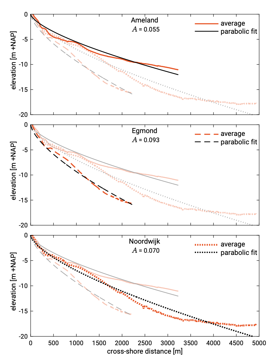
Before discussing the importance of the dynamic equilibrium concept for engineering applications we need to know how accurate the predictive ability is. We therefore apply a parabolic fit to the three earlier presented (Fig. 7.5) typical profiles along the Dutch coast, knowing that these profiles differ considerably (see Figs. 7.7 and 7.8). Two profiles are from the Holland coast, one in the southern section and one in the northern section and one from the Wadden Sea coast (in all cases \(D_{50}\) = approximately \(200\ \mu m\)). The fits were made to the average profile over the 55 yearly measurements. Note that the expression \(h = A(x)^m\) results in a vertical slope of the beach profile at the waterline (\(x' = 0\)). This is not realistic. In practical applications it should be considered to position this point at a level somewhere above the waterline (1 m in our example). This results in more reasonable slopes at the waterline. Furthermore, we need to define the offshore extent of the profile fit, for which one may adopt the active zone concept as defined by Hallermeier (1978) who introduced the concept of depth of closure (Fig. 1.14). In his definition the active zone corresponds to the surf zone width for extreme conditions exceeded twelve hours per year.
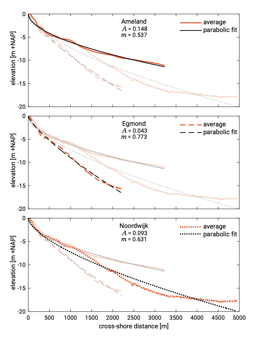
Even though the mean grain diameter is the same for all three locations, the optimal values of \(A\) with fixed power \(m = 2/3\) (see Fig. 7.2.2.7 and Table 7.1) nearly differ a factor of 2! According to Eq. 7.2.2.7 the value of \(A\) should be 0.10 (based on a fall velocity \(w_s = 0.0256\ m/s\)). These results indicate that the predictive ability of Eq. 7.2.2.1 is limited. We hypothesise that the value of \(A\) is not only dependent on the fall velocity but also on several other variables, like wave climate, tide and surge water level variations and coastal currents. Hence, care must be taken with the accuracy of Eq. 7.2.2.1 for engineering applications. Obviously, a fit with two free parameters improves the fit somewhat (Fig. 7.8), but the variation in the values of \(A\) is even larger and the theoretical foundation is lacking.
Nonetheless, the dynamic equilibrium concept is one of the few tools that a coastal engineer has available to make a prediction of the expected profile of a new land reclamation or a newly constructed offshore island. A particularly useful application concerns the expected changes in the dynamic equilibrium profile when a coast is nourished with borrow sediment sizes that differ from the native sediment size. Dean (2002) discusses this application at length, summarizing most of his earlier work.
| A (Eq. 7.2.2.7) | A (Ameland) | A (Egmond) | A (Noordwijk) |
| 0.10 | 0.055 | 0.093 | 0.070 |