6.2.3: Fall velocity
- Page ID
- 16346
\( \newcommand{\vecs}[1]{\overset { \scriptstyle \rightharpoonup} {\mathbf{#1}} } \)
\( \newcommand{\vecd}[1]{\overset{-\!-\!\rightharpoonup}{\vphantom{a}\smash {#1}}} \)
\( \newcommand{\id}{\mathrm{id}}\) \( \newcommand{\Span}{\mathrm{span}}\)
( \newcommand{\kernel}{\mathrm{null}\,}\) \( \newcommand{\range}{\mathrm{range}\,}\)
\( \newcommand{\RealPart}{\mathrm{Re}}\) \( \newcommand{\ImaginaryPart}{\mathrm{Im}}\)
\( \newcommand{\Argument}{\mathrm{Arg}}\) \( \newcommand{\norm}[1]{\| #1 \|}\)
\( \newcommand{\inner}[2]{\langle #1, #2 \rangle}\)
\( \newcommand{\Span}{\mathrm{span}}\)
\( \newcommand{\id}{\mathrm{id}}\)
\( \newcommand{\Span}{\mathrm{span}}\)
\( \newcommand{\kernel}{\mathrm{null}\,}\)
\( \newcommand{\range}{\mathrm{range}\,}\)
\( \newcommand{\RealPart}{\mathrm{Re}}\)
\( \newcommand{\ImaginaryPart}{\mathrm{Im}}\)
\( \newcommand{\Argument}{\mathrm{Arg}}\)
\( \newcommand{\norm}[1]{\| #1 \|}\)
\( \newcommand{\inner}[2]{\langle #1, #2 \rangle}\)
\( \newcommand{\Span}{\mathrm{span}}\) \( \newcommand{\AA}{\unicode[.8,0]{x212B}}\)
\( \newcommand{\vectorA}[1]{\vec{#1}} % arrow\)
\( \newcommand{\vectorAt}[1]{\vec{\text{#1}}} % arrow\)
\( \newcommand{\vectorB}[1]{\overset { \scriptstyle \rightharpoonup} {\mathbf{#1}} } \)
\( \newcommand{\vectorC}[1]{\textbf{#1}} \)
\( \newcommand{\vectorD}[1]{\overrightarrow{#1}} \)
\( \newcommand{\vectorDt}[1]{\overrightarrow{\text{#1}}} \)
\( \newcommand{\vectE}[1]{\overset{-\!-\!\rightharpoonup}{\vphantom{a}\smash{\mathbf {#1}}}} \)
\( \newcommand{\vecs}[1]{\overset { \scriptstyle \rightharpoonup} {\mathbf{#1}} } \)
\( \newcommand{\vecd}[1]{\overset{-\!-\!\rightharpoonup}{\vphantom{a}\smash {#1}}} \)
\(\newcommand{\avec}{\mathbf a}\) \(\newcommand{\bvec}{\mathbf b}\) \(\newcommand{\cvec}{\mathbf c}\) \(\newcommand{\dvec}{\mathbf d}\) \(\newcommand{\dtil}{\widetilde{\mathbf d}}\) \(\newcommand{\evec}{\mathbf e}\) \(\newcommand{\fvec}{\mathbf f}\) \(\newcommand{\nvec}{\mathbf n}\) \(\newcommand{\pvec}{\mathbf p}\) \(\newcommand{\qvec}{\mathbf q}\) \(\newcommand{\svec}{\mathbf s}\) \(\newcommand{\tvec}{\mathbf t}\) \(\newcommand{\uvec}{\mathbf u}\) \(\newcommand{\vvec}{\mathbf v}\) \(\newcommand{\wvec}{\mathbf w}\) \(\newcommand{\xvec}{\mathbf x}\) \(\newcommand{\yvec}{\mathbf y}\) \(\newcommand{\zvec}{\mathbf z}\) \(\newcommand{\rvec}{\mathbf r}\) \(\newcommand{\mvec}{\mathbf m}\) \(\newcommand{\zerovec}{\mathbf 0}\) \(\newcommand{\onevec}{\mathbf 1}\) \(\newcommand{\real}{\mathbb R}\) \(\newcommand{\twovec}[2]{\left[\begin{array}{r}#1 \\ #2 \end{array}\right]}\) \(\newcommand{\ctwovec}[2]{\left[\begin{array}{c}#1 \\ #2 \end{array}\right]}\) \(\newcommand{\threevec}[3]{\left[\begin{array}{r}#1 \\ #2 \\ #3 \end{array}\right]}\) \(\newcommand{\cthreevec}[3]{\left[\begin{array}{c}#1 \\ #2 \\ #3 \end{array}\right]}\) \(\newcommand{\fourvec}[4]{\left[\begin{array}{r}#1 \\ #2 \\ #3 \\ #4 \end{array}\right]}\) \(\newcommand{\cfourvec}[4]{\left[\begin{array}{c}#1 \\ #2 \\ #3 \\ #4 \end{array}\right]}\) \(\newcommand{\fivevec}[5]{\left[\begin{array}{r}#1 \\ #2 \\ #3 \\ #4 \\ #5 \\ \end{array}\right]}\) \(\newcommand{\cfivevec}[5]{\left[\begin{array}{c}#1 \\ #2 \\ #3 \\ #4 \\ #5 \\ \end{array}\right]}\) \(\newcommand{\mattwo}[4]{\left[\begin{array}{rr}#1 \amp #2 \\ #3 \amp #4 \\ \end{array}\right]}\) \(\newcommand{\laspan}[1]{\text{Span}\{#1\}}\) \(\newcommand{\bcal}{\cal B}\) \(\newcommand{\ccal}{\cal C}\) \(\newcommand{\scal}{\cal S}\) \(\newcommand{\wcal}{\cal W}\) \(\newcommand{\ecal}{\cal E}\) \(\newcommand{\coords}[2]{\left\{#1\right\}_{#2}}\) \(\newcommand{\gray}[1]{\color{gray}{#1}}\) \(\newcommand{\lgray}[1]{\color{lightgray}{#1}}\) \(\newcommand{\rank}{\operatorname{rank}}\) \(\newcommand{\row}{\text{Row}}\) \(\newcommand{\col}{\text{Col}}\) \(\renewcommand{\row}{\text{Row}}\) \(\newcommand{\nul}{\text{Nul}}\) \(\newcommand{\var}{\text{Var}}\) \(\newcommand{\corr}{\text{corr}}\) \(\newcommand{\len}[1]{\left|#1\right|}\) \(\newcommand{\bbar}{\overline{\bvec}}\) \(\newcommand{\bhat}{\widehat{\bvec}}\) \(\newcommand{\bperp}{\bvec^\perp}\) \(\newcommand{\xhat}{\widehat{\xvec}}\) \(\newcommand{\vhat}{\widehat{\vvec}}\) \(\newcommand{\uhat}{\widehat{\uvec}}\) \(\newcommand{\what}{\widehat{\wvec}}\) \(\newcommand{\Sighat}{\widehat{\Sigma}}\) \(\newcommand{\lt}{<}\) \(\newcommand{\gt}{>}\) \(\newcommand{\amp}{&}\) \(\definecolor{fillinmathshade}{gray}{0.9}\)
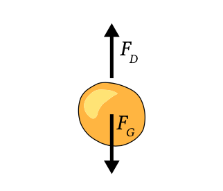
When a particle falls in still and clear water, it accelerates until it reaches a constant vertical velocity that is called fall velocity or settling velocity. This velocity can be assessed from the balance between the downward directed gravity force \(F_G\) (minus the effect of buoyancy) and the upward directed (retarding) drag force \(F_D\) as indicated in Fig. 6.1.
Basic equation
The downward directed gravity force \(F_G\) on a sphere combined with the upward buoyancy effect is given by the so-called underwater weight of the sphere, viz. by the weight of the sphere minus the weight of the displaced volume of water. With weight equal to mass times acceleration due to gravity, we have for a perfect sphere:
\[F_G = (\rho_s - \rho) g \left (\dfrac{\pi}{6} D^3 \right )\]
where:
| \(\rho_s\) | mass density of the particle | \(kg/m^3\) |
| \(\rho\) | mass density of the surrounding fluid | \(kg/m^3\) |
| \(D\) | particle diameter | \(m\) |
| \(g\) | acceleration of gravity | \(m/s^2\) |
In this equation, the term between the brackets is the volume of the sphere.
The upward directed force is equal to the so-called drag force denoted by:
\[F_D = \dfrac{1}{2} C_D \rho w_s^2 \left (\dfrac{\pi}{4} D^2 \right )\]
where:
| \(C_D\) | drag coefficient | |
| \(w_s\) | particle fall velocity | \(m/s\) |
The second term between the brackets refers to the cross-section of the sphere. The drag force is non-zero only if \(w_s > 0\).
In equilibrium, both forces are in balance and the fall velocity \(w_s\) (in \(m/s\)) is given by:
\[w_s = \sqrt{\dfrac{4(s - 1) gD}{3C_D}}\label{eq6.2.3.3}\]
in which \(s\) is the relative density (see Sect. 6.2.2).
A particle’s fall velocity depends on its size, its density and on the magnitude of the drag coefficient \(C_D\). This drag coefficient depends on the shape of the particle, its roughness but mainly on the grain Reynolds number:
\[\text{Re} = w_s D/v\]
where
| \(v\) | kinematic viscosity coefficient | \(m^2/s\) |
The kinematic viscosity is defined as the dynamic viscosity divided by the water density: \(v = \mu /\rho\). A characteristic value for \(v\) is \(10^{-6}\ m^2/s\). The dynamic viscosity represents the fluid’s internal resistance to flow (‘thickness’) and is a function of the temperature and to a smaller extent of the density.
Dependence on Reynolds number

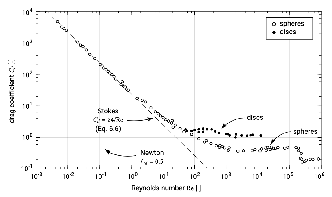
For low grain Reynolds numbers (\(\text{Re} < 0.1\) to 0.5 ) in the so-called Stokes-range, the drag coefficient can be described by (see Fig. 6.2):
\[C_D = 24/\text{Re}\]
yielding:
\[w_s = \dfrac{(s - 1) gD^2}{18v}\]
In this range, the fall velocity depends on the square of the grain diameter, the relative density and the kinematic viscosity coefficient.
For high grain Reynolds numbers (\(400 < Re < 2 \times 10^5\)), in the so-called Newton range, the drag coefficient becomes a constant (\(C_D \approx 0.5\)). In that case it follows from Eq. \(\ref{eq6.2.3.3}\):
\[w_s = 1.6 \sqrt{gD(s - 1)}\]
In this range, the fall velocity depends on the square root of the grain diameter and the relative density and is independent of the kinematic viscosity coefficient. This is also the case for extremely high Reynolds numbers (\(\text{Re} > 2 \times 10^5\)), where the drag coefficient is (constant) around 0.2.
For quartz spheres falling in still water, a Reynolds number of 0.5 corresponds roughly with a particle diameter of 0.08 mm, while a Reynolds number of 400 corresponds with a diameter of about 1.9 mm. Since most beach sediments fall in the range of 0.08 mm to 1.9 mm, in most practical cases neither the Stokes approximation nor the Newton approximation can be used.

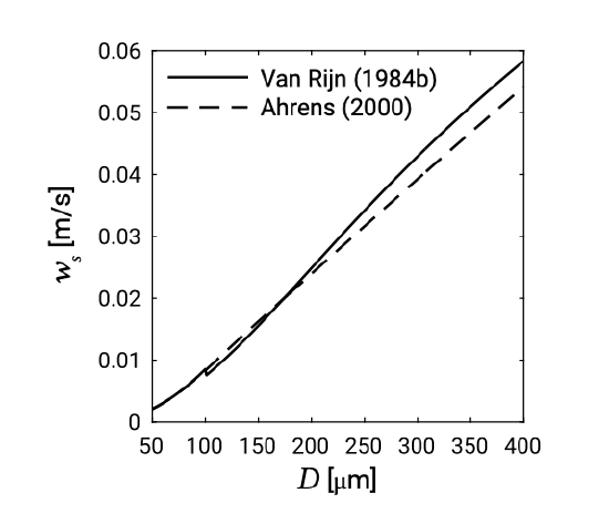
For very small particles (silt, clay) the fall velocity is proportional to \(D^2\); for gravel size particles the fall velocity is proportional to \(\sqrt{D}\). For sand, the fall velocity falls in the transition range between a \(D^2\) dependency and a \(\sqrt{D}\) dependency. By lack of a simple relationship for the drag coefficient in this range, it is common practice to use empirical formulas for the fall velocity. In literature, many formulas can be found (e.g. Van Rijn (1984b) and Ahrens (2000)). As an example, in Fig. 6.3, for two formulas the fall velocity as a function of the grain diameter is plotted.
Hindered settling
In high concentration mixtures the fall velocity of a single particle is reduced due to the presence of other particles. This can be explained as follows: with each downward grain movement, a similar fluid volume must flow upward; this upward flow slows down the other grains. In order to account for this hindered settling effect, the fall velocity in a fluid-sediment mixture should be determined as a function of the sediment concentration \(c\) and the particle fall velocity \(w_s\). An often used formulation for the effective fall velocity in a mixture is:
\[w_e = (1 - c)^{\alpha} w_s\]
where:
| \(w_e\) | effective fall velocity | \(m/s\) |
| \(w_s\) | fall velocity of one grain in clear water in rest | \(m/s\) |
| \(c\) | sediment concentration (volumetric %, volume of solid sediment particles in volume of water-sediment mixture) | - |
| \(\alpha\) | coefficient (ranging from 4.6 at low Reynolds numbers to 2.3 at high Reynolds numbers) | - |
In many engineering cases related to sediment transport, the sediment concentration can be up to approximately 1% (\(2.65\ kg/m^3\)), meaning that the effect of sediment concentration on the fall velocity is small. This is not the case in sheet-flow conditions (see Sect. 6.4.2) and in very silty environments where sediment concentrations can be significantly higher.


