
6.6.3: Time-averaged concentration distribution
- Page ID
- 16359

\( \newcommand{\vecs}[1]{\overset { \scriptstyle \rightharpoonup} {\mathbf{#1}} } \)
\( \newcommand{\vecd}[1]{\overset{-\!-\!\rightharpoonup}{\vphantom{a}\smash {#1}}} \)
\( \newcommand{\dsum}{\displaystyle\sum\limits} \)
\( \newcommand{\dint}{\displaystyle\int\limits} \)
\( \newcommand{\dlim}{\displaystyle\lim\limits} \)
\( \newcommand{\id}{\mathrm{id}}\) \( \newcommand{\Span}{\mathrm{span}}\)
( \newcommand{\kernel}{\mathrm{null}\,}\) \( \newcommand{\range}{\mathrm{range}\,}\)
\( \newcommand{\RealPart}{\mathrm{Re}}\) \( \newcommand{\ImaginaryPart}{\mathrm{Im}}\)
\( \newcommand{\Argument}{\mathrm{Arg}}\) \( \newcommand{\norm}[1]{\| #1 \|}\)
\( \newcommand{\inner}[2]{\langle #1, #2 \rangle}\)
\( \newcommand{\Span}{\mathrm{span}}\)
\( \newcommand{\id}{\mathrm{id}}\)
\( \newcommand{\Span}{\mathrm{span}}\)
\( \newcommand{\kernel}{\mathrm{null}\,}\)
\( \newcommand{\range}{\mathrm{range}\,}\)
\( \newcommand{\RealPart}{\mathrm{Re}}\)
\( \newcommand{\ImaginaryPart}{\mathrm{Im}}\)
\( \newcommand{\Argument}{\mathrm{Arg}}\)
\( \newcommand{\norm}[1]{\| #1 \|}\)
\( \newcommand{\inner}[2]{\langle #1, #2 \rangle}\)
\( \newcommand{\Span}{\mathrm{span}}\) \( \newcommand{\AA}{\unicode[.8,0]{x212B}}\)
\( \newcommand{\vectorA}[1]{\vec{#1}} % arrow\)
\( \newcommand{\vectorAt}[1]{\vec{\text{#1}}} % arrow\)
\( \newcommand{\vectorB}[1]{\overset { \scriptstyle \rightharpoonup} {\mathbf{#1}} } \)
\( \newcommand{\vectorC}[1]{\textbf{#1}} \)
\( \newcommand{\vectorD}[1]{\overrightarrow{#1}} \)
\( \newcommand{\vectorDt}[1]{\overrightarrow{\text{#1}}} \)
\( \newcommand{\vectE}[1]{\overset{-\!-\!\rightharpoonup}{\vphantom{a}\smash{\mathbf {#1}}}} \)
\( \newcommand{\vecs}[1]{\overset { \scriptstyle \rightharpoonup} {\mathbf{#1}} } \)
\(\newcommand{\longvect}{\overrightarrow}\)
\( \newcommand{\vecd}[1]{\overset{-\!-\!\rightharpoonup}{\vphantom{a}\smash {#1}}} \)
\(\newcommand{\avec}{\mathbf a}\) \(\newcommand{\bvec}{\mathbf b}\) \(\newcommand{\cvec}{\mathbf c}\) \(\newcommand{\dvec}{\mathbf d}\) \(\newcommand{\dtil}{\widetilde{\mathbf d}}\) \(\newcommand{\evec}{\mathbf e}\) \(\newcommand{\fvec}{\mathbf f}\) \(\newcommand{\nvec}{\mathbf n}\) \(\newcommand{\pvec}{\mathbf p}\) \(\newcommand{\qvec}{\mathbf q}\) \(\newcommand{\svec}{\mathbf s}\) \(\newcommand{\tvec}{\mathbf t}\) \(\newcommand{\uvec}{\mathbf u}\) \(\newcommand{\vvec}{\mathbf v}\) \(\newcommand{\wvec}{\mathbf w}\) \(\newcommand{\xvec}{\mathbf x}\) \(\newcommand{\yvec}{\mathbf y}\) \(\newcommand{\zvec}{\mathbf z}\) \(\newcommand{\rvec}{\mathbf r}\) \(\newcommand{\mvec}{\mathbf m}\) \(\newcommand{\zerovec}{\mathbf 0}\) \(\newcommand{\onevec}{\mathbf 1}\) \(\newcommand{\real}{\mathbb R}\) \(\newcommand{\twovec}[2]{\left[\begin{array}{r}#1 \\ #2 \end{array}\right]}\) \(\newcommand{\ctwovec}[2]{\left[\begin{array}{c}#1 \\ #2 \end{array}\right]}\) \(\newcommand{\threevec}[3]{\left[\begin{array}{r}#1 \\ #2 \\ #3 \end{array}\right]}\) \(\newcommand{\cthreevec}[3]{\left[\begin{array}{c}#1 \\ #2 \\ #3 \end{array}\right]}\) \(\newcommand{\fourvec}[4]{\left[\begin{array}{r}#1 \\ #2 \\ #3 \\ #4 \end{array}\right]}\) \(\newcommand{\cfourvec}[4]{\left[\begin{array}{c}#1 \\ #2 \\ #3 \\ #4 \end{array}\right]}\) \(\newcommand{\fivevec}[5]{\left[\begin{array}{r}#1 \\ #2 \\ #3 \\ #4 \\ #5 \\ \end{array}\right]}\) \(\newcommand{\cfivevec}[5]{\left[\begin{array}{c}#1 \\ #2 \\ #3 \\ #4 \\ #5 \\ \end{array}\right]}\) \(\newcommand{\mattwo}[4]{\left[\begin{array}{rr}#1 \amp #2 \\ #3 \amp #4 \\ \end{array}\right]}\) \(\newcommand{\laspan}[1]{\text{Span}\{#1\}}\) \(\newcommand{\bcal}{\cal B}\) \(\newcommand{\ccal}{\cal C}\) \(\newcommand{\scal}{\cal S}\) \(\newcommand{\wcal}{\cal W}\) \(\newcommand{\ecal}{\cal E}\) \(\newcommand{\coords}[2]{\left\{#1\right\}_{#2}}\) \(\newcommand{\gray}[1]{\color{gray}{#1}}\) \(\newcommand{\lgray}[1]{\color{lightgray}{#1}}\) \(\newcommand{\rank}{\operatorname{rank}}\) \(\newcommand{\row}{\text{Row}}\) \(\newcommand{\col}{\text{Col}}\) \(\renewcommand{\row}{\text{Row}}\) \(\newcommand{\nul}{\text{Nul}}\) \(\newcommand{\var}{\text{Var}}\) \(\newcommand{\corr}{\text{corr}}\) \(\newcommand{\len}[1]{\left|#1\right|}\) \(\newcommand{\bbar}{\overline{\bvec}}\) \(\newcommand{\bhat}{\widehat{\bvec}}\) \(\newcommand{\bperp}{\bvec^\perp}\) \(\newcommand{\xhat}{\widehat{\xvec}}\) \(\newcommand{\vhat}{\widehat{\vvec}}\) \(\newcommand{\uhat}{\widehat{\uvec}}\) \(\newcommand{\what}{\widehat{\wvec}}\) \(\newcommand{\Sighat}{\widehat{\Sigma}}\) \(\newcommand{\lt}{<}\) \(\newcommand{\gt}{>}\) \(\newcommand{\amp}{&}\) \(\definecolor{fillinmathshade}{gray}{0.9}\)In a steady situation \(\partial c/ \partial t = 0\) and \(c = C\). A balance must exist between the upward transport by turbulence and the downward transport with the fall velocity. Integration of Eq. 6.6.2.6 over the depth (with a zero vertical flux at the water surface) leads to:
\[w_s C(z) + v_{t,s} (z) \dfrac{dC(z)}{dz} = 0\label{eq6.6.3.1}\]
This equation indicates an equilibrium between the downward transport with the fall velocity \(w_s C(z)\) and the net upward movement of grains by turbulence.
As mentioned above, local turbulence in the water column leads to an upward and a downward exchange of sediment-laden fluid parcels. Since the sediment concentration is larger close to the bed, more grains will be transported in the upward direction than in the downward direction. This leads to a turbulent transport of sediment, which depends on the gradient in concentration over the vertical. This is why it is referred to as a gradient-type transport. On average, turbulence transports sediment from levels of high concentrations to levels of lower concentrations, i.e. from lower levels in the water column to higher levels.
Generally the suspended sediment is somewhat finer than the bed material. Hence, in order to compute the constant fall velocity often a smaller grain diameter is used than in the computation of the bed load transport.
The assumption of upward transport due to turbulent diffusion seems reasonable for a plane bed. In the situation of a rippled bed however, it can be expected that upward transport is by eddies generated by the ripples (see Intermezzo 6.1). These are coherent fluid motions that bring the sediment upward by convection. In that case, the whole concept of upward transport proportional to a concentration gradient does not hold anymore. Sometimes, the diffusion concept is stretched a bit by assuming that the sediment diffusivity accounts for the convection processes also.
It makes sense to relate the turbulent diffusivity \(v_{t, s}\) of sediment mass to the eddy viscosity of the fluid through a factor \(\beta\): \(v_{t,s} = \beta v_t\). A value of \(\beta < 1\) reflects that the sediment particles cannot respond fully to the turbulent fluid velocity fluctuations (inertia). On the other hand \(\beta > 1\) (supported by laboratory experiments) indicates a more effective mixing for sediment particles than for water particles. It has been argued that this is the result of larger centrifugal forces on sediment particles in eddies than on fluid particles (because of their higher density). In the following \(\beta = 1\) is used.
With an appropriate distribution for \(v_{t, s}\) (for which many candidates exist in literature!) and a bottom boundary condition, Eq. \(\ref{eq6.6.3.1}\) can be integrated either numerically or analytically. Analytical solutions are possible for simple diffusivity distributions.
The integration is performed from a near-bed reference level \(a\) to the water surface. At the reference level \(a\) concentration-type boundary condition can be used. Since in principle \(z = a\) corresponds to the top of the bed load layer, the reference concentration must be somehow related to the bed load transport rate, for instance via:
\[C_a = \dfrac{S_b}{ua}\]
where:
| \(S_b\) | bed load transport | \(m^3/m/s\) |
| \(u\) | average fluid velocity in the bottom layer | \(m/s\) |
| \(a\) | thickness of the bottom layer (order of magnitude of the bottom roughness \(r\)) | \(m\) |
The reference concentration is often formulated as a function of the time-averaged bed shear stress and should take the enhanced stirring by waves into account.
The most general solution of Eq. \(\ref{eq6.6.3.1}\) is:
\[C(z) = C_a \exp \left [-\int_{z = a}^{z} \dfrac{w_s}{v_{t, s} (z)} dz \right ]\]
where:
| \(C_a\) | time-mean concentration at level \(z = a\) | - |
| \(w_s\) | fall velocity | \(m/s\) |
| \(z\) | height above the bed | \(m\) |
Einstein (1942, 1950) and Rouse (1937) suggested a parabolic distribution of the diffusion coefficient over the water depth:
\[v_{t,s} (z) = \kappa u_* \dfrac{z}{h} (h - z)\]
where:
| \(\kappa\) | Von Karman constant = 0.4 |
A parabolic sediment diffusivity is in accordance with the generally assumed parabolic eddy viscosity in the water column (increasing from zero at the ‘walls’ to a maximum away from the walls, see Eq. 5.5.5.17 and the text below it).
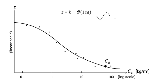
This results in the following concentration distribution (see Fig. 6.16):
\[C(z) = C_a \left [\dfrac{h - z}{z} \dfrac{a}{h - a} \right ]^{z_*}\]
where:
| \(a\) | thickness of the bottom layer | \(m\) |
| \(C_a\) | concentration at reference level \(z = a\) | - |
| \(z_*\) | Rouse number defined as \(z_* = \dfrac{w_s}{\kappa u_*}\) | - |
The Rouse number is a non-dimensional number that not only defines the sediment concentration profile, but also determines the mode of transport. It is the ratio between the downward sediment fall velocity and the upwards velocity on the grain represented by \(\kappa u_*\). For Rouse numbers larger than, say, 2.5 (or \(w_s/u_* > 1\)) all transport is bed load transport. For a Rouse number smaller than, say, 0.8, we have only wash load. Between these extremes sediment suspension occurs. If \(w_s/u_* > 1\) we may say that the sediment is coarse and responds quasi-steadily to the flow field. For \(w_s/u_* < 1\) (‘fine’ sand in suspension) non-instantaneous sediment responses start playing a role.