3.6: Long term statistics and extreme values

As indicated above, waves are measured at regular intervals of 3 to 6 hours during a relatively short period during which the record can be considered stationary. This results in a series of wave observations with sampling interval of 3 or 6 hours. If long enough (years or even decades, as in the case of the Dutch wave data), this series can in its turn be considered a set of random data representing the long-term wave climate of the location. Not only measured wave climates are used for this, but also hindcasts based on archived wind fields. Note that for periods of decades, conditions may not be stationary (due to for instance climate change impacts on wave climate).

For many engineering problems long-term statistics of average parameters are sufficient. The long term data can be represented in various ways:

• Histograms of \(H_s\) present the percentage of occurrence of a certain significant wave height.
• Scatter plots of \(H_s\) versus wave period show the dependency of wave periods and wave heights.
• Tables can include information on wave period and wave angle also, for instance a table valid for a certain direction sector which gives the percentage of occurrence of \(H_s\) versus \(\overline{T_0}\).
• Wave roses give the directional distribution of the wave heights.

Mostly, long-term distributions of significant wave heights are determined, which present \(H_s\) versus the percentage of exceedance. Long-term distributions of wave peri- ods and wave angles can also be determined but are often considered to be a function of the long-term wave height distribution. Sometimes the long-term distribution functions for \(H_s\) are calculated for different wave angle classes.

Since extreme conditions are not always part of observed data, extrapolation is some- times needed. For extrapolation of the probabilities several distributions can be used. The choice does not have a theoretical basis. Often used are the log-normal distribution and the Weibull distribution. These analyses will not give information on when an event will happen but it is possible to determine how often it is likely happen.

The percentage of exceedance can also be expressed as a return period. The return period is defined as the average time between events with a (significant) wave height larger than a certain value.

Figure 3.15: Wave climate for the validation case in Table 3.3 presented as a wave rose.

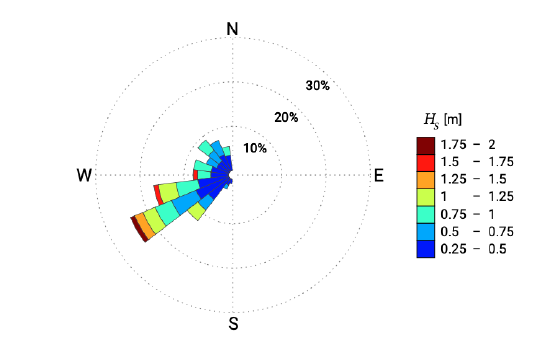
For an engineering project the wave climate is generally known at some distance from the coastal site. We can then use a wave model to translate this offshore wave climate to a climate representative for the project site. However, a full wave climate consists of a multitude of wave conditions, which is often not practical. An example of a year-averaged wave climate based on a wave study is shown in Table 3.3 and Fig. 3.15. Instead of using all those conditions in morphodynamic computations, often engineers reduce such a climate to a representative set with fewer conditions. But what is representative in this context? That depends on the problem under consideration. For an engineering problem which is governed by longshore sediment transport a representative set of wave conditions means that at least the total longshore transport rate reproduced by the smaller set is identical to the rate based on the full climate. After such a wave climate schematisation, morphodynamic computations can be carried out for fewer conditions, which is therefore faster.

Table 3.3: Wave conditions for validation case. From Mol (2007)

condition	\(H_s\) [m]	dir [\(^{\circ}N\)]	\(T_p\) [s]	duration [%]	days/yr
1	0.4	188	2.85	1.00	3.65
2	0.4	203	2.85	1.50	5.48
3	0.6	203	3.49	1.00	3.65
4	0.4	218	2.85	6.00	21.9
5	0.6	218	3.49	3.00	10.95
6	1.2	218	4.93	3.00	10.95
7	1.8	233	6.04	1.00	3.65
8	1.4	233	5.32	2.00	7.4
9	1.0	233	4.50	3.00	10.95
10	0.8	233	4.02	4.00	14.6
11	0.6	233	3.49	6.00	21.9
12	0.4	233	2.85	8.00	29.2
13	0.4	248	2.85	7.00	25.55
14	0.8	248	4.02	5.00	18.25
15	1.2	248	4.93	4.00	14.6
16	1.6	248	5.69	1.00	3.65
17	1.6	263	5.69	1.00	3.65
18	0.8	263	4.02	3.00	10.95
19	0.4	263	2.85	4.00	14.6
20	0.8	278	4.02	4.00	14.6
21	0.4	278	2.85	4.00	14.6
22	0.4	293	2.85	3.00	10.95
23	0.6	293	3.49	2.50	9.13
24	0.8	308	4.02	3.00	10.95
25	0.6	308	3.49	3.00	10.95
26	0.4	308	2.85	3.00	10.95
27	0.6	323	3.49	3.50	12.78
28	0.4	323	2.85	4.00	14.6
29	0.4	338	2.85	3.50	10.95
30	0.8	338	4.02	2.00	9.13
total				100	365

For applications like determining the height of a deck of a platform, the probabilities of individual wave heights are required. In such cases, the short term and the long-term expectations must be combined to obtain the probability of exceedance of individual wave heights during a fixed period, for example the lifetime of the structure. This also is often close to a Weibull distribution.

Because in shallow water there is a direct relation between maximum breaking wave height and water depth, the wave height distribution is not independent of the occurrence of extreme water levels. Close to the shore, this could mean that the long-term distribution of wave heights coincides with the distribution of extreme water levels.