1.5.3: Time and spatial scales
- Page ID
- 16255
\( \newcommand{\vecs}[1]{\overset { \scriptstyle \rightharpoonup} {\mathbf{#1}} } \)
\( \newcommand{\vecd}[1]{\overset{-\!-\!\rightharpoonup}{\vphantom{a}\smash {#1}}} \)
\( \newcommand{\id}{\mathrm{id}}\) \( \newcommand{\Span}{\mathrm{span}}\)
( \newcommand{\kernel}{\mathrm{null}\,}\) \( \newcommand{\range}{\mathrm{range}\,}\)
\( \newcommand{\RealPart}{\mathrm{Re}}\) \( \newcommand{\ImaginaryPart}{\mathrm{Im}}\)
\( \newcommand{\Argument}{\mathrm{Arg}}\) \( \newcommand{\norm}[1]{\| #1 \|}\)
\( \newcommand{\inner}[2]{\langle #1, #2 \rangle}\)
\( \newcommand{\Span}{\mathrm{span}}\)
\( \newcommand{\id}{\mathrm{id}}\)
\( \newcommand{\Span}{\mathrm{span}}\)
\( \newcommand{\kernel}{\mathrm{null}\,}\)
\( \newcommand{\range}{\mathrm{range}\,}\)
\( \newcommand{\RealPart}{\mathrm{Re}}\)
\( \newcommand{\ImaginaryPart}{\mathrm{Im}}\)
\( \newcommand{\Argument}{\mathrm{Arg}}\)
\( \newcommand{\norm}[1]{\| #1 \|}\)
\( \newcommand{\inner}[2]{\langle #1, #2 \rangle}\)
\( \newcommand{\Span}{\mathrm{span}}\) \( \newcommand{\AA}{\unicode[.8,0]{x212B}}\)
\( \newcommand{\vectorA}[1]{\vec{#1}} % arrow\)
\( \newcommand{\vectorAt}[1]{\vec{\text{#1}}} % arrow\)
\( \newcommand{\vectorB}[1]{\overset { \scriptstyle \rightharpoonup} {\mathbf{#1}} } \)
\( \newcommand{\vectorC}[1]{\textbf{#1}} \)
\( \newcommand{\vectorD}[1]{\overrightarrow{#1}} \)
\( \newcommand{\vectorDt}[1]{\overrightarrow{\text{#1}}} \)
\( \newcommand{\vectE}[1]{\overset{-\!-\!\rightharpoonup}{\vphantom{a}\smash{\mathbf {#1}}}} \)
\( \newcommand{\vecs}[1]{\overset { \scriptstyle \rightharpoonup} {\mathbf{#1}} } \)
\( \newcommand{\vecd}[1]{\overset{-\!-\!\rightharpoonup}{\vphantom{a}\smash {#1}}} \)
\(\newcommand{\avec}{\mathbf a}\) \(\newcommand{\bvec}{\mathbf b}\) \(\newcommand{\cvec}{\mathbf c}\) \(\newcommand{\dvec}{\mathbf d}\) \(\newcommand{\dtil}{\widetilde{\mathbf d}}\) \(\newcommand{\evec}{\mathbf e}\) \(\newcommand{\fvec}{\mathbf f}\) \(\newcommand{\nvec}{\mathbf n}\) \(\newcommand{\pvec}{\mathbf p}\) \(\newcommand{\qvec}{\mathbf q}\) \(\newcommand{\svec}{\mathbf s}\) \(\newcommand{\tvec}{\mathbf t}\) \(\newcommand{\uvec}{\mathbf u}\) \(\newcommand{\vvec}{\mathbf v}\) \(\newcommand{\wvec}{\mathbf w}\) \(\newcommand{\xvec}{\mathbf x}\) \(\newcommand{\yvec}{\mathbf y}\) \(\newcommand{\zvec}{\mathbf z}\) \(\newcommand{\rvec}{\mathbf r}\) \(\newcommand{\mvec}{\mathbf m}\) \(\newcommand{\zerovec}{\mathbf 0}\) \(\newcommand{\onevec}{\mathbf 1}\) \(\newcommand{\real}{\mathbb R}\) \(\newcommand{\twovec}[2]{\left[\begin{array}{r}#1 \\ #2 \end{array}\right]}\) \(\newcommand{\ctwovec}[2]{\left[\begin{array}{c}#1 \\ #2 \end{array}\right]}\) \(\newcommand{\threevec}[3]{\left[\begin{array}{r}#1 \\ #2 \\ #3 \end{array}\right]}\) \(\newcommand{\cthreevec}[3]{\left[\begin{array}{c}#1 \\ #2 \\ #3 \end{array}\right]}\) \(\newcommand{\fourvec}[4]{\left[\begin{array}{r}#1 \\ #2 \\ #3 \\ #4 \end{array}\right]}\) \(\newcommand{\cfourvec}[4]{\left[\begin{array}{c}#1 \\ #2 \\ #3 \\ #4 \end{array}\right]}\) \(\newcommand{\fivevec}[5]{\left[\begin{array}{r}#1 \\ #2 \\ #3 \\ #4 \\ #5 \\ \end{array}\right]}\) \(\newcommand{\cfivevec}[5]{\left[\begin{array}{c}#1 \\ #2 \\ #3 \\ #4 \\ #5 \\ \end{array}\right]}\) \(\newcommand{\mattwo}[4]{\left[\begin{array}{rr}#1 \amp #2 \\ #3 \amp #4 \\ \end{array}\right]}\) \(\newcommand{\laspan}[1]{\text{Span}\{#1\}}\) \(\newcommand{\bcal}{\cal B}\) \(\newcommand{\ccal}{\cal C}\) \(\newcommand{\scal}{\cal S}\) \(\newcommand{\wcal}{\cal W}\) \(\newcommand{\ecal}{\cal E}\) \(\newcommand{\coords}[2]{\left\{#1\right\}_{#2}}\) \(\newcommand{\gray}[1]{\color{gray}{#1}}\) \(\newcommand{\lgray}[1]{\color{lightgray}{#1}}\) \(\newcommand{\rank}{\operatorname{rank}}\) \(\newcommand{\row}{\text{Row}}\) \(\newcommand{\col}{\text{Col}}\) \(\renewcommand{\row}{\text{Row}}\) \(\newcommand{\nul}{\text{Nul}}\) \(\newcommand{\var}{\text{Var}}\) \(\newcommand{\corr}{\text{corr}}\) \(\newcommand{\len}[1]{\left|#1\right|}\) \(\newcommand{\bbar}{\overline{\bvec}}\) \(\newcommand{\bhat}{\widehat{\bvec}}\) \(\newcommand{\bperp}{\bvec^\perp}\) \(\newcommand{\xhat}{\widehat{\xvec}}\) \(\newcommand{\vhat}{\widehat{\vvec}}\) \(\newcommand{\uhat}{\widehat{\uvec}}\) \(\newcommand{\what}{\widehat{\wvec}}\) \(\newcommand{\Sighat}{\widehat{\Sigma}}\) \(\newcommand{\lt}{<}\) \(\newcommand{\gt}{>}\) \(\newcommand{\amp}{&}\) \(\definecolor{fillinmathshade}{gray}{0.9}\)
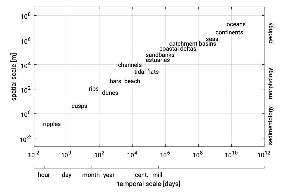
As we have seen in the previous two sections, the behaviour of a natural coastal system is dynamic on a variety of time and spatial scales. The spatial scale is generally determined by the dimensions (in m) of a particular morphological element; it indicates the extent of the element. Examples of spatial scales (see also Fig. 1.17) are:
- A whole tidal inlet system, comprising of a flood basin, an inlet gorge and an ebb or outer delta. Dimensions vary between 50 to 700 \(km^2\). Morphological changes on such a large spatial scale generally take decades to centuries (e.g. the gradual migration of the entire inlet system);
- Large tidal channels and sand banks. Typical surface dimensions are 5 to 20 \(km^2\), while significant changes generally take place within years to decades (such as the landing of the sand bank ‘De Onrust’ on the south coast of Texel around 1910);
- Smaller tidal channels and bars, with typical surface dimensions of maximum several \(km^2\). Significant morphological changes occur within years (such as the development and landing of the ‘Bornrif’ sand bar on the west coast of Ameland in the nineties of the last century);
- Accretion and erosion patterns at both sides of a port entrance, built with the help of long breakwaters. The spatial scale is several kilometres;
- Smaller bed forms like ripples and (bottom) dunes. The related spatial scales are as small as metres or less.
Figure 1.17 suggests that spatial and timescales are closely coupled; the larger the spatial scale of a certain feature, the larger the timescale. As an example, smaller bed forms (as mentioned in the last bullet of the above bullet list) not only have small spatial scales but also small timescales; the time periods in which significant changes occur are less than days.
| Morphological unit | Basin that is abruptly closed | Surface area of flood basin after closure [\(km^2\)] | Observed morphological time scale [year] |
| Outer delta Haringvliet | Haringvliet (1970) | 120 | 11 |
| Zoutkamperlaag | Lauwerszee (1969) | 200 | 17 |
| Outer delta Texel Inlet | Zuiderzee (1932) | 680 | 32 |
Examples of morphological timescales are given in Table 1.1. These examples are related to the observed morphological changes of the outer deltas of several Dutch tidal inlet systems after abrupt changes in their flood basins. The figures support the general idea that morphological timescales are directly coupled to the spatial scales of the morphological units.
A timescale is generally interpreted as the period of time (e.g. in years) required for characteristic morphological developments. Some researchers relate the timescale to the total duration that a morphological system needs to reach a new equilibrium situation once it has been disturbed by nature or by man (see Sect. 1.5.4). Equilibrium in this sense means that the overall sediment balance of the morphological unit is maintained (no erosion and no accretion).
A coastal engineer would generally not be interested in dynamics on very small scales like the evolution of wave ripples on the seabed or even breaker bars in the surf zone (see Sect. 1.4.2). The dynamics on these scales are generally oscillatory, which means that they have no net effect on engineering timescales. By contrast, the natural behaviour on larger (human/engineering) scales generally shows a net trend. Examples are depth reduction of an estuary due to infilling by sediments, the erosion or accretion of a delta, and the migration of a tidal inlet. Human interventions have timescales of years to decades and spatial scales of 1 km to 100 km. The coastal behaviour due to human interventions (harbours, coastal defence works, land reclamation) interferes with the natural behaviour of the coastal system on these time and spatial scales.
Long-term sea-level change acts on timescales larger than engineering scales (order of ten thousand years). This long-term tendency needs to be taken into account in the analysis on the engineering scale of the system; it provides boundary conditions for processes and system evolution on the engineering scale. Coastal evolution on geological timescales (such as plate tectonics) is responsible for the large-scale geographical variation of coastal systems that we find around the globe nowadays. These large-scale characteristics can be considered as a given for any analysis on engineering timescales. In Ch. 2 we discuss this distribution of coastal environments and – briefly – its origin.


