
5.6.2: Biaxial Interference Figures
- Page ID
- 19131

\( \newcommand{\vecs}[1]{\overset { \scriptstyle \rightharpoonup} {\mathbf{#1}} } \)
\( \newcommand{\vecd}[1]{\overset{-\!-\!\rightharpoonup}{\vphantom{a}\smash {#1}}} \)
\( \newcommand{\dsum}{\displaystyle\sum\limits} \)
\( \newcommand{\dint}{\displaystyle\int\limits} \)
\( \newcommand{\dlim}{\displaystyle\lim\limits} \)
\( \newcommand{\id}{\mathrm{id}}\) \( \newcommand{\Span}{\mathrm{span}}\)
( \newcommand{\kernel}{\mathrm{null}\,}\) \( \newcommand{\range}{\mathrm{range}\,}\)
\( \newcommand{\RealPart}{\mathrm{Re}}\) \( \newcommand{\ImaginaryPart}{\mathrm{Im}}\)
\( \newcommand{\Argument}{\mathrm{Arg}}\) \( \newcommand{\norm}[1]{\| #1 \|}\)
\( \newcommand{\inner}[2]{\langle #1, #2 \rangle}\)
\( \newcommand{\Span}{\mathrm{span}}\)
\( \newcommand{\id}{\mathrm{id}}\)
\( \newcommand{\Span}{\mathrm{span}}\)
\( \newcommand{\kernel}{\mathrm{null}\,}\)
\( \newcommand{\range}{\mathrm{range}\,}\)
\( \newcommand{\RealPart}{\mathrm{Re}}\)
\( \newcommand{\ImaginaryPart}{\mathrm{Im}}\)
\( \newcommand{\Argument}{\mathrm{Arg}}\)
\( \newcommand{\norm}[1]{\| #1 \|}\)
\( \newcommand{\inner}[2]{\langle #1, #2 \rangle}\)
\( \newcommand{\Span}{\mathrm{span}}\) \( \newcommand{\AA}{\unicode[.8,0]{x212B}}\)
\( \newcommand{\vectorA}[1]{\vec{#1}} % arrow\)
\( \newcommand{\vectorAt}[1]{\vec{\text{#1}}} % arrow\)
\( \newcommand{\vectorB}[1]{\overset { \scriptstyle \rightharpoonup} {\mathbf{#1}} } \)
\( \newcommand{\vectorC}[1]{\textbf{#1}} \)
\( \newcommand{\vectorD}[1]{\overrightarrow{#1}} \)
\( \newcommand{\vectorDt}[1]{\overrightarrow{\text{#1}}} \)
\( \newcommand{\vectE}[1]{\overset{-\!-\!\rightharpoonup}{\vphantom{a}\smash{\mathbf {#1}}}} \)
\( \newcommand{\vecs}[1]{\overset { \scriptstyle \rightharpoonup} {\mathbf{#1}} } \)
\(\newcommand{\longvect}{\overrightarrow}\)
\( \newcommand{\vecd}[1]{\overset{-\!-\!\rightharpoonup}{\vphantom{a}\smash {#1}}} \)
\(\newcommand{\avec}{\mathbf a}\) \(\newcommand{\bvec}{\mathbf b}\) \(\newcommand{\cvec}{\mathbf c}\) \(\newcommand{\dvec}{\mathbf d}\) \(\newcommand{\dtil}{\widetilde{\mathbf d}}\) \(\newcommand{\evec}{\mathbf e}\) \(\newcommand{\fvec}{\mathbf f}\) \(\newcommand{\nvec}{\mathbf n}\) \(\newcommand{\pvec}{\mathbf p}\) \(\newcommand{\qvec}{\mathbf q}\) \(\newcommand{\svec}{\mathbf s}\) \(\newcommand{\tvec}{\mathbf t}\) \(\newcommand{\uvec}{\mathbf u}\) \(\newcommand{\vvec}{\mathbf v}\) \(\newcommand{\wvec}{\mathbf w}\) \(\newcommand{\xvec}{\mathbf x}\) \(\newcommand{\yvec}{\mathbf y}\) \(\newcommand{\zvec}{\mathbf z}\) \(\newcommand{\rvec}{\mathbf r}\) \(\newcommand{\mvec}{\mathbf m}\) \(\newcommand{\zerovec}{\mathbf 0}\) \(\newcommand{\onevec}{\mathbf 1}\) \(\newcommand{\real}{\mathbb R}\) \(\newcommand{\twovec}[2]{\left[\begin{array}{r}#1 \\ #2 \end{array}\right]}\) \(\newcommand{\ctwovec}[2]{\left[\begin{array}{c}#1 \\ #2 \end{array}\right]}\) \(\newcommand{\threevec}[3]{\left[\begin{array}{r}#1 \\ #2 \\ #3 \end{array}\right]}\) \(\newcommand{\cthreevec}[3]{\left[\begin{array}{c}#1 \\ #2 \\ #3 \end{array}\right]}\) \(\newcommand{\fourvec}[4]{\left[\begin{array}{r}#1 \\ #2 \\ #3 \\ #4 \end{array}\right]}\) \(\newcommand{\cfourvec}[4]{\left[\begin{array}{c}#1 \\ #2 \\ #3 \\ #4 \end{array}\right]}\) \(\newcommand{\fivevec}[5]{\left[\begin{array}{r}#1 \\ #2 \\ #3 \\ #4 \\ #5 \\ \end{array}\right]}\) \(\newcommand{\cfivevec}[5]{\left[\begin{array}{c}#1 \\ #2 \\ #3 \\ #4 \\ #5 \\ \end{array}\right]}\) \(\newcommand{\mattwo}[4]{\left[\begin{array}{rr}#1 \amp #2 \\ #3 \amp #4 \\ \end{array}\right]}\) \(\newcommand{\laspan}[1]{\text{Span}\{#1\}}\) \(\newcommand{\bcal}{\cal B}\) \(\newcommand{\ccal}{\cal C}\) \(\newcommand{\scal}{\cal S}\) \(\newcommand{\wcal}{\cal W}\) \(\newcommand{\ecal}{\cal E}\) \(\newcommand{\coords}[2]{\left\{#1\right\}_{#2}}\) \(\newcommand{\gray}[1]{\color{gray}{#1}}\) \(\newcommand{\lgray}[1]{\color{lightgray}{#1}}\) \(\newcommand{\rank}{\operatorname{rank}}\) \(\newcommand{\row}{\text{Row}}\) \(\newcommand{\col}{\text{Col}}\) \(\renewcommand{\row}{\text{Row}}\) \(\newcommand{\nul}{\text{Nul}}\) \(\newcommand{\var}{\text{Var}}\) \(\newcommand{\corr}{\text{corr}}\) \(\newcommand{\len}[1]{\left|#1\right|}\) \(\newcommand{\bbar}{\overline{\bvec}}\) \(\newcommand{\bhat}{\widehat{\bvec}}\) \(\newcommand{\bperp}{\bvec^\perp}\) \(\newcommand{\xhat}{\widehat{\xvec}}\) \(\newcommand{\vhat}{\widehat{\vvec}}\) \(\newcommand{\uhat}{\widehat{\uvec}}\) \(\newcommand{\what}{\widehat{\wvec}}\) \(\newcommand{\Sighat}{\widehat{\Sigma}}\) \(\newcommand{\lt}{<}\) \(\newcommand{\gt}{>}\) \(\newcommand{\amp}{&}\) \(\definecolor{fillinmathshade}{gray}{0.9}\)We obtain biaxial interference figures in the same way as uniaxial interference figures. However, complications arise with biaxial minerals because it is more difficult to find and identify grains oriented in a useful way. We can get interference figures from all grains, but interpreting them can be difficult or impossible.
With care, however, we can identify three different kinds of useful figures: optic axis figures (OA), acute bisectrix figures (Bxa), and optic normal figures (ON). Each corresponds to a different light path through the crystal, relative to the orientation of the optic axes. A fourth type of figure – a Bxo figure (Bxo) – is generally of limited use but we discuss it briefly in the interests of thoroughness.
Figure 5.69 shows the orientations of the different views for a typical biaxial mineral. The optic plane is vertical in the drawing on the left, but is horizontal in the drawing on the right. You can compare these drawings with ones seen earlier in which the crystallographic (a, b, c) and optical axes (X, Y, and Z) were labeled (Figures 5.60 and 5.61).
Video 11: Biaxial interference figures with good photos (5 minutes)
5.6.2.1 Optic Axis Figure
We obtain an OA figure by looking down an optic axis (Figure 5.69). We can find grains oriented to give an OA figure because they have zero or extremely low retardation. Under normal XP light, they remain dark even when we rotate the microscope stage. An interference figure will show only one isogyre unless 2V is quite small (less than 30°).
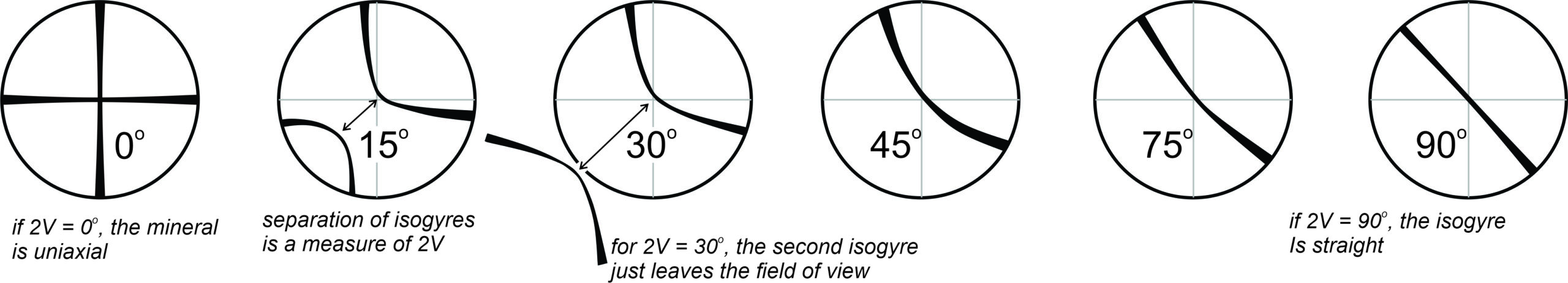
Figure 5.70 show depictions of isogyres for different values of 2V. (In these drawings, the isogyres are narrow with sharp boundaries but in thin section they are commonly quite diffuse.) No matter the 2V value, if the figure is perfectly centered, the isogyres will remain centered with stage rotation. If 2V = 0o it means we are looking at a uniaxial mineral and we see a black cross. If 2V is very low (< 30̊o) We will see two isogyres, shown in the 15o drawing above. The two isogyres will come together and separate with stage rotation. If 2V > 30o the second isogyre no longer enters the field of view. As 2V approaches 90o, the single isogyre becomes straighter, and at 90o the isogyre is completely straight. So, the curvature allows us to estimate 2V.
For any value of 2V, stage rotation causes isogyre rotation. For some purposes, discussed later, we may wish to know which side of the isogyre is concave and which is convex; this can be difficult to discern if 2V is very large because the isogyre will be nearly straight. In part also, the difficulty arises because a straight biaxial isogyre (unlike a uniaxial isogyre) does not have to be parallel or perpendicular to the microscope crosshairs.
Video 12: Link to an optic axis figure for betrandite (biaxial) (30 seconds)
5.6.2.2 Bxa and Bxo Figures
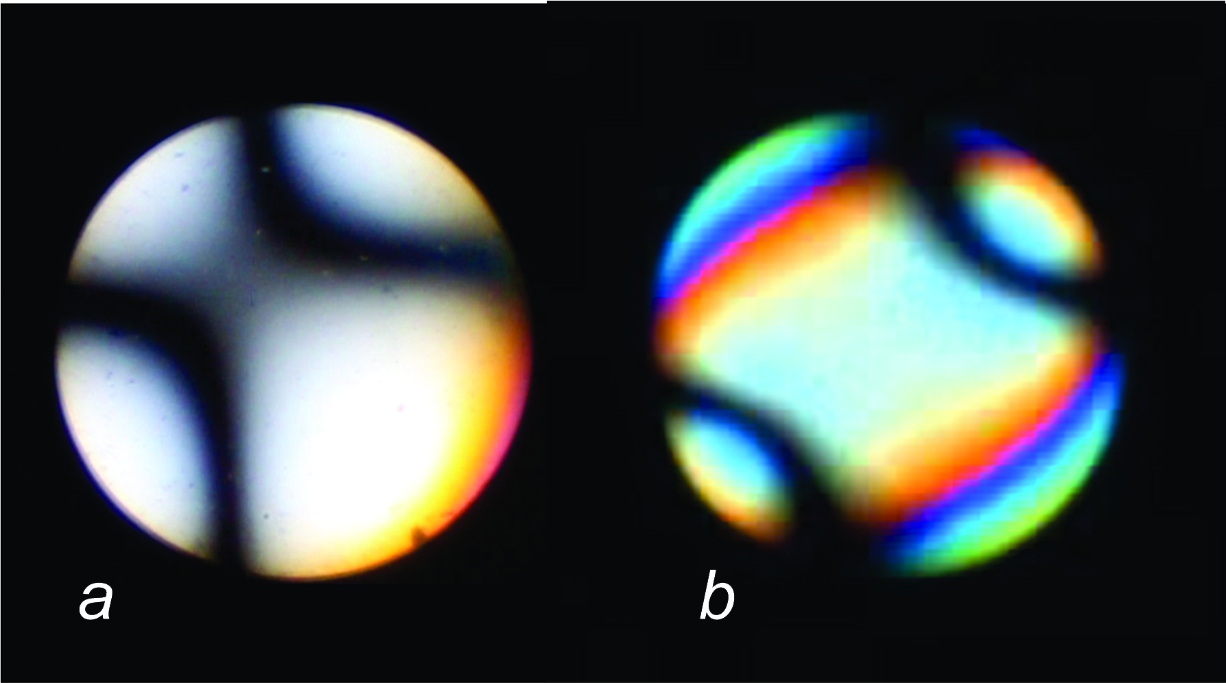
We obtain Bxa figures, such as those in Figure 5.71 by looking down the acute bisectrix, the line bisecting the acute angle between the two optic axes (Figure 5.69). We obtain a Bxo figure by looking down the obtuse bisectrix, the line bisecting the obtuse angle between the two optic axes (Figure 5.69). In biaxial positive crystals, Bxa corresponds to a view along Z; in biaxial negative crystals, it corresponds to a view along X. The opposite is true for Bxo figures. Generally, however, we do not seek a Bxo figure because it is of less use than a Bxa. So the discussion below focuses mostly on Bxas.
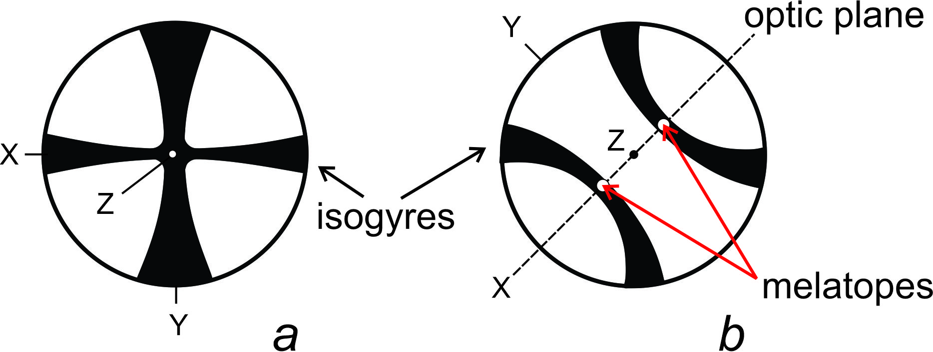
When we observe an acute bisectrix figure (Bxa) for a grain in an extinction orientation (which occurs when Y is perpendicular to a polarizer), it appears as a black cross, similar in some respects to a uniaxial interference figure (Figure 5.72a). When we rotate the stage, the cross splits into two isogyres that move apart and may leave the field of view (Figure 5.72b). After a rotation of 45°, the isogyres are at maximum separation; they come back together to reform the cross every 90°.
The points on the isogyres closest to the center of a Bxa (or a Bxo), the melatopes, are points corresponding to the orientations of the optic axes (Figure 5.72b). (Figure 5.72b is for a biaxial positive crystal; X and Z will switch places for a biaxial negative crystal.) If the retardation of the crystal is large enough, isochromes circle the melatopes. Some colorful isochromes are apparent in Figure 5.71b, above. Isochrome interference colors increase in order moving away from the melatopes because retardation is greater as the angle to the optic axes increases.
In Figure 5.71a, the isogyres are just beginning to separate; in Figure 5.71b they are at maximum separation. The maximum amount of isogyre separation depends on 2V; the greater the separation, the larger the 2V. If 2V is less than about 60°, the isogyres of a well-centered figure stay in the field of view as we rotate the stage. If 2V is greater than 60°, the isogyres completely leave the field of view
Finding a grain that yields a Bxa is easiest for minerals with a small 2V. We begin by searching for a grain that has minimal retardation. Such a grain will be oriented with an optical axis near vertical. Then we obtain an interference figure. We rotate the stage, and note how the isogyres behave. After checking several grains, we will find a Bxa. For minerals with low-to-moderate 2V, both isogyres will stay in the field of view, but the interference figure may not be perfectly centered. If an isogyre leaves the field of view, we check other grains until we are sure we are looking at a nearly centered Bxa. Getting a perfectly centered Bxo or Bxa figure can be, however, difficult and, sometimes for off-centered figures, we may only see one isogyre clearly.
For minerals with high 2V, the search for a Bxa sometimes becomes frustrating. Distinguishing a Bxa from a Bxo may be difficult or impossible. If we mistake one for the other, we may get some properties, 2V for example, wrong if we make measurements. But, the isogyres in a Bxo figure always leave the field of view because, by definition, an obtuse angle separates the optic axes in the Bxo direction. Thus, if the isogyres remain in view, the figure is a Bxa figure. For standard lenses, if the isogyres leave the field of view, the figure may be a Bxo or a Bxa for a mineral with high 2V (greater than about 60°). Expert optical mineralogists can tell a Bxa from a Bxo figure by the speed with which the isogyre leaves the field of view on stage rotation. For the rest of us, it is probably best to search for another grain with a better orientation.
Video 13: Link to off-center Bxa figure for titanite (30 seconds)
5.6.2.3 Optic Normal Figure (ON)
We get an optic normal (ON) figure by looking down Y, normal to the plane of the two optic axes (see Figures 5.60 and 5.61). Grains that yield an optic normal figure are those that have maximum retardation, which means maximum interference colors. The interference figure resembles a poorly resolved Bxa, but the isogyres leave the field of view with only a slight rotation of the stage. Biaxial optic normal figures appear similar to uniaxial flash figures.
5.6.2.4 Determining Optic Sign and 2V of a Biaxial Mineral
Determining optic sign from a Bxa figure is equivalent to asking whether the Bxa view is parallel to the fast direction (biaxial negative crystals) or to the slow direction (biaxial positive crystals). We can often make the determination in much the same manner as for a uniaxial optic axis figure. However, for figures where the isogyres leave the field of view, this is not the recommended method because we can easily confuse Bxa and Bxo figures when 2V is greater than 70° or 80°. An alternative way to learn optic sign and 2V is to find a grain that yields a centered optic axis figure. Finding such grains is often not difficult because they show very low-order interference colors, or may appear isotropic under crossed polars. Below, we discuss both methods.
5.6.2.5 Determining Sign and 2V from a Bxa Figure
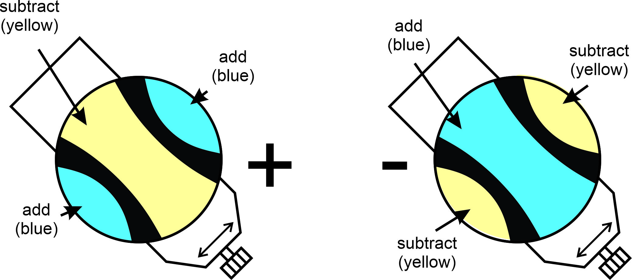
To measure optic sign and 2V using a Bxa figure, we rotate the stage so the isogyres are in the southwest and northeast quadrants (Figure 5.73). The Y direction in the crystal is now oriented northwest-southeast. The points corresponding to the optic axes (the melatopes) are the points on the isogyres closest to each other, and either X or Z is vertical depending on optic sign.
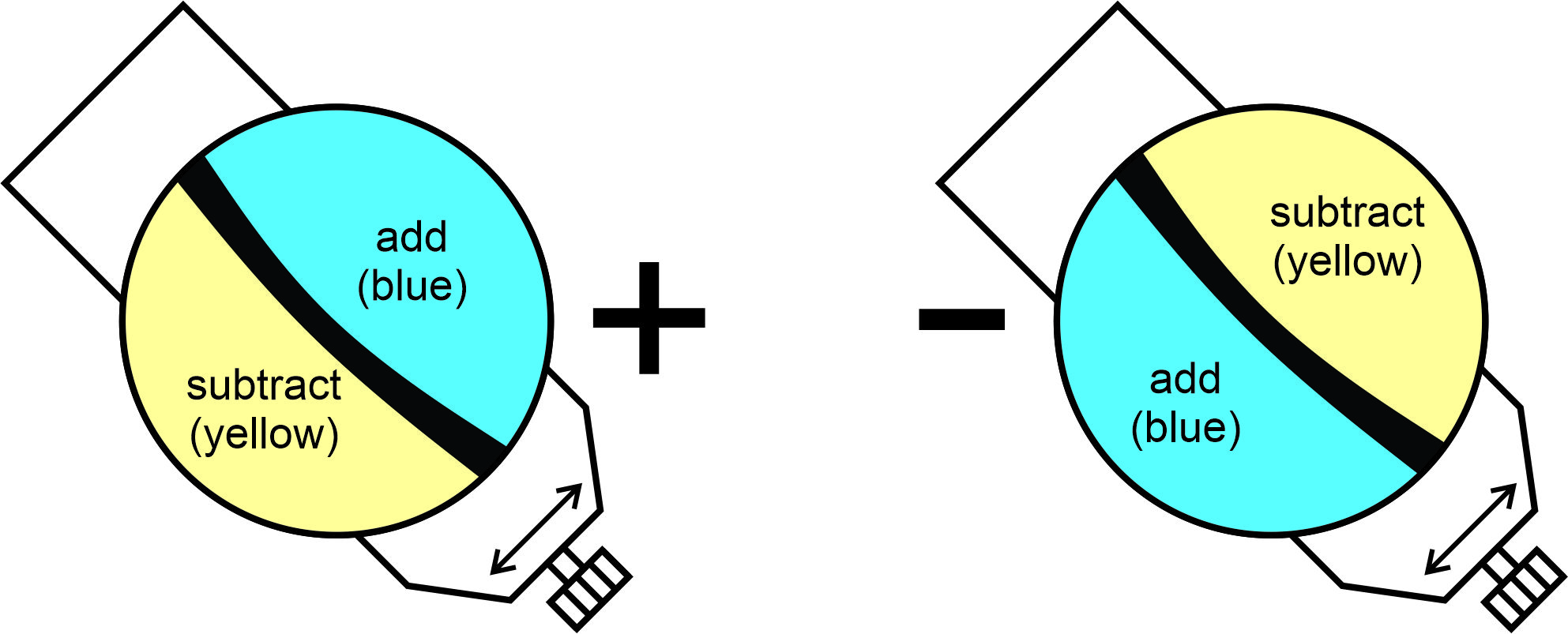
To determine optic sign, we must know which direction (X or Z) is vertical, corresponding to Bxa. If the slow direction (Z) corresponds to Bxa, the crystal is positive. If the fast direction (X) is Bxa, the crystal is negative. To make the determination, we insert the full-wave accessory plate (with slow-oriented direction southwest-northeast) and note any changes in interference colors on the concave sides of the isogyres. If the interference colors add on the concave sides of the isogyres (and subtract on the convex sides), the mineral is positive (Figure 5.73).
In positive minerals with low to moderate retardation, the colors in the center of the figure will be yellow (subtraction), and those on the concave side of the isogyres will be blue (addition). In a negative mineral, the color changes will be the opposite. For minerals with high retardation, it may be difficult to decide whether a full-wave accessory plate adds or subtracts retardation because isochromes of many repeating colors circle the melatopes. A quartz wedge simplifies determination. As we insert the wedge, color rings move toward the melatopes if there is addition of retardation, or the rings move away from the melatopes if there is subtraction. If the interference colors move toward the optic axes from the concave side of the isogyres, and away on the convex side, the mineral is positive. We see the opposite effect for a negative mineral.
We can estimate 2V from a well-centered Bxa figure by noting the maximum of separation of the isogyres during stage rotation. For standard lenses, if the isogyres just leave the field of view when they are at maximum separation, 2V is 60° to 65°. If the isogyres barely separate, 2V is less than about 10°.
5.6.2.6 Determining Sign and 2V from an Optic Axis Figure
Determining the optic sign from an optic axis figure can often be simpler than looking for a Bxa. To find an OA figure, we look for a grain displaying zero or very low retardation. Once we have an interference figure, we rotate the stage and we should see one centered or nearly centered isogyre (Figures 5.70). (If, instead, we see two isogyres that stay in the field of view when we rotate the stage, we are looking at a Bxa for a mineral with low 2V.) We rotate the stage so the isogyre (or the most nearly centered if there are two isogyres) is concave to the northeast (Figure 5.74). Note that isogyres rotate in the opposite sense from the stage.
We then insert the full-wave accessory plate. If the retardation increases on the concave side of the isogyre (and decreases on the convex side), the mineral is positive (Figures 5.74). In minerals with low to moderate retardation, we need only to look for yellow and blue. Blue indicates an increase and yellow a decrease in retardation. The increase or decrease of retardation will be opposite if the mineral is negative.
We estimate 2V by noting the curvature of the isogyre. If 2V is less than 10° to 15°, the isogyre will seem to make a 90° bend. If 2V is 90°, it will be straight. For other values, it will have curvature between 90° and 0° (Figure 5.70).