
2.8: Interference Figures
- Page ID
- 11109

\( \newcommand{\vecs}[1]{\overset { \scriptstyle \rightharpoonup} {\mathbf{#1}} } \)
\( \newcommand{\vecd}[1]{\overset{-\!-\!\rightharpoonup}{\vphantom{a}\smash {#1}}} \)
\( \newcommand{\id}{\mathrm{id}}\) \( \newcommand{\Span}{\mathrm{span}}\)
( \newcommand{\kernel}{\mathrm{null}\,}\) \( \newcommand{\range}{\mathrm{range}\,}\)
\( \newcommand{\RealPart}{\mathrm{Re}}\) \( \newcommand{\ImaginaryPart}{\mathrm{Im}}\)
\( \newcommand{\Argument}{\mathrm{Arg}}\) \( \newcommand{\norm}[1]{\| #1 \|}\)
\( \newcommand{\inner}[2]{\langle #1, #2 \rangle}\)
\( \newcommand{\Span}{\mathrm{span}}\)
\( \newcommand{\id}{\mathrm{id}}\)
\( \newcommand{\Span}{\mathrm{span}}\)
\( \newcommand{\kernel}{\mathrm{null}\,}\)
\( \newcommand{\range}{\mathrm{range}\,}\)
\( \newcommand{\RealPart}{\mathrm{Re}}\)
\( \newcommand{\ImaginaryPart}{\mathrm{Im}}\)
\( \newcommand{\Argument}{\mathrm{Arg}}\)
\( \newcommand{\norm}[1]{\| #1 \|}\)
\( \newcommand{\inner}[2]{\langle #1, #2 \rangle}\)
\( \newcommand{\Span}{\mathrm{span}}\) \( \newcommand{\AA}{\unicode[.8,0]{x212B}}\)
\( \newcommand{\vectorA}[1]{\vec{#1}} % arrow\)
\( \newcommand{\vectorAt}[1]{\vec{\text{#1}}} % arrow\)
\( \newcommand{\vectorB}[1]{\overset { \scriptstyle \rightharpoonup} {\mathbf{#1}} } \)
\( \newcommand{\vectorC}[1]{\textbf{#1}} \)
\( \newcommand{\vectorD}[1]{\overrightarrow{#1}} \)
\( \newcommand{\vectorDt}[1]{\overrightarrow{\text{#1}}} \)
\( \newcommand{\vectE}[1]{\overset{-\!-\!\rightharpoonup}{\vphantom{a}\smash{\mathbf {#1}}}} \)
\( \newcommand{\vecs}[1]{\overset { \scriptstyle \rightharpoonup} {\mathbf{#1}} } \)
\( \newcommand{\vecd}[1]{\overset{-\!-\!\rightharpoonup}{\vphantom{a}\smash {#1}}} \)
\(\newcommand{\avec}{\mathbf a}\) \(\newcommand{\bvec}{\mathbf b}\) \(\newcommand{\cvec}{\mathbf c}\) \(\newcommand{\dvec}{\mathbf d}\) \(\newcommand{\dtil}{\widetilde{\mathbf d}}\) \(\newcommand{\evec}{\mathbf e}\) \(\newcommand{\fvec}{\mathbf f}\) \(\newcommand{\nvec}{\mathbf n}\) \(\newcommand{\pvec}{\mathbf p}\) \(\newcommand{\qvec}{\mathbf q}\) \(\newcommand{\svec}{\mathbf s}\) \(\newcommand{\tvec}{\mathbf t}\) \(\newcommand{\uvec}{\mathbf u}\) \(\newcommand{\vvec}{\mathbf v}\) \(\newcommand{\wvec}{\mathbf w}\) \(\newcommand{\xvec}{\mathbf x}\) \(\newcommand{\yvec}{\mathbf y}\) \(\newcommand{\zvec}{\mathbf z}\) \(\newcommand{\rvec}{\mathbf r}\) \(\newcommand{\mvec}{\mathbf m}\) \(\newcommand{\zerovec}{\mathbf 0}\) \(\newcommand{\onevec}{\mathbf 1}\) \(\newcommand{\real}{\mathbb R}\) \(\newcommand{\twovec}[2]{\left[\begin{array}{r}#1 \\ #2 \end{array}\right]}\) \(\newcommand{\ctwovec}[2]{\left[\begin{array}{c}#1 \\ #2 \end{array}\right]}\) \(\newcommand{\threevec}[3]{\left[\begin{array}{r}#1 \\ #2 \\ #3 \end{array}\right]}\) \(\newcommand{\cthreevec}[3]{\left[\begin{array}{c}#1 \\ #2 \\ #3 \end{array}\right]}\) \(\newcommand{\fourvec}[4]{\left[\begin{array}{r}#1 \\ #2 \\ #3 \\ #4 \end{array}\right]}\) \(\newcommand{\cfourvec}[4]{\left[\begin{array}{c}#1 \\ #2 \\ #3 \\ #4 \end{array}\right]}\) \(\newcommand{\fivevec}[5]{\left[\begin{array}{r}#1 \\ #2 \\ #3 \\ #4 \\ #5 \\ \end{array}\right]}\) \(\newcommand{\cfivevec}[5]{\left[\begin{array}{c}#1 \\ #2 \\ #3 \\ #4 \\ #5 \\ \end{array}\right]}\) \(\newcommand{\mattwo}[4]{\left[\begin{array}{rr}#1 \amp #2 \\ #3 \amp #4 \\ \end{array}\right]}\) \(\newcommand{\laspan}[1]{\text{Span}\{#1\}}\) \(\newcommand{\bcal}{\cal B}\) \(\newcommand{\ccal}{\cal C}\) \(\newcommand{\scal}{\cal S}\) \(\newcommand{\wcal}{\cal W}\) \(\newcommand{\ecal}{\cal E}\) \(\newcommand{\coords}[2]{\left\{#1\right\}_{#2}}\) \(\newcommand{\gray}[1]{\color{gray}{#1}}\) \(\newcommand{\lgray}[1]{\color{lightgray}{#1}}\) \(\newcommand{\rank}{\operatorname{rank}}\) \(\newcommand{\row}{\text{Row}}\) \(\newcommand{\col}{\text{Col}}\) \(\renewcommand{\row}{\text{Row}}\) \(\newcommand{\nul}{\text{Nul}}\) \(\newcommand{\var}{\text{Var}}\) \(\newcommand{\corr}{\text{corr}}\) \(\newcommand{\len}[1]{\left|#1\right|}\) \(\newcommand{\bbar}{\overline{\bvec}}\) \(\newcommand{\bhat}{\widehat{\bvec}}\) \(\newcommand{\bperp}{\bvec^\perp}\) \(\newcommand{\xhat}{\widehat{\xvec}}\) \(\newcommand{\vhat}{\widehat{\vvec}}\) \(\newcommand{\uhat}{\widehat{\uvec}}\) \(\newcommand{\what}{\widehat{\wvec}}\) \(\newcommand{\Sighat}{\widehat{\Sigma}}\) \(\newcommand{\lt}{<}\) \(\newcommand{\gt}{>}\) \(\newcommand{\amp}{&}\) \(\definecolor{fillinmathshade}{gray}{0.9}\)Interference figures are a technique which can be used to help identify minerals using a polarizing light microscope. In this chapter, we explore the practical aspects of obtaining and interpreting interference figures and other related observations.
Learning Objectives
Students should be able to:
- Describe the steps used to obtain interference figures.
- Correctly name the parts of an interference figure.
- Describe the features of an indicatrix.
- Identify the type of interference figure produced.
- Connect crystal symmetry to the type of interference figure(s) that are produced.
- Use interference figures to narrow down the possible symmetry choices and help identify a mineral.
- Make optical sign determinations and 2V angle estimates to further help identify minerals (optional).
How to Obtain an Interference Figure
These videos show the steps to obtaining an interference figure. They are shot at two different angles so it is possible to see the operation of the microscope better.
What is a Bertrand Lens? See section 2.4 to review!
In each of these videos, there is a single mineral crystal on the slide. If you are looking at multiple grains of the same mineral, you may find it helpful tolocate mineral grains with the lowest interference colors (lowest retardation) to obtain interference figures that are the easiest to identify (e.g., uniaxial optic axes figures, or biaxial acute bisectrix figures, which will be described below).
Figure \(\PageIndex{2}\)
Question 2.8.1. Drag and drop the steps of obtaining an interference figure in the correct order.
Anatomy of an Interference Figure
Below is an example of one type of interference figure. This figure contains three types of features: isogyres, a melatope, and isochromes.
Figure \(\PageIndex{3}\)
Figure 2.8.3. Anatomy of an interference figure.
The Indicatrix
The index of refraction is different in different crystallographic directions within a mineral, according to its crystal symmetry. We can characterize this using an ellipsoid (roughly the shape of an American football or rugby ball-shaped object) which shows the refractive index in every direction, including the three principle optical axes. This ellipsoid is called an indicatrix.
The indicatrix is a 3-dimensional visualization of the indices of refraction of a mineral. As discussed previously in light and optics, the index of refraction is different for different minerals. It can also vary as a function of direction within the crystal structure. Minerals with lower symmetries have greater variation in the index of refraction with direction.
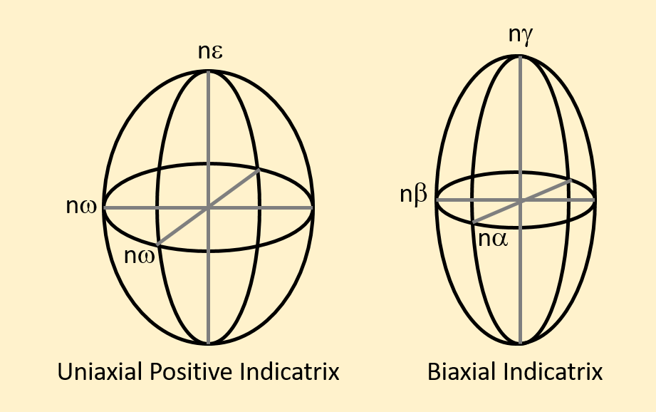
As discussed in Section 2.3 Light and Optics, Birefringence, a solid material such as a mineral can split light waves into two polarized beams, the ordinary ray (represented by “o” or “ω” and the extraordinary ray (represented by “e” or “ε”). Uniaxial minerals exhibit the same refractive index along two principal axes (nω), and a different refractive index along the third principal axis (nε). Biaxial minerals have different refractive index values along each principal axis, with nα as the lowest refractive index, nβ as an intermediate refractive index, and nγ as the largest refractive index.
Why create this type of diagram? It is useful for thinking about how the interference figure will vary as the crystal is oriented in different directions in the thin section. Indicatrices are shown in the figures showing uniaxial and biaxial interference figures in the sections below. The figures show the orientation of the indices of refraction with respect to the thin section surface using the indicatrix, and the resulting interference figure.
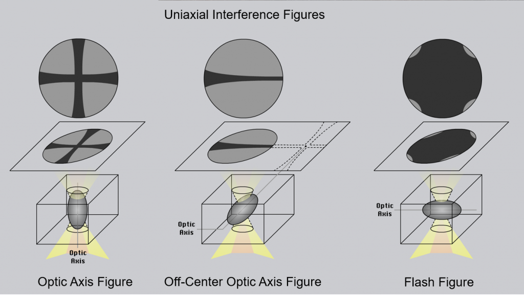
Uniaxial Interference Figures
The following two videos explain how to obtain uniaxial interference figures and how to determine optic sign for a uniaxial mineral. Figure 2.8.7 summarizes the types of interference figures that can be observed for uniaxial minerals.
Guided Inquiry
Biaxial Interference Figures
The following two videos explain how to obtain biaxial interference figures, how to determine optic sign for a biaxial mineral, and how to estimate a 2V angle.
Biaxial interference figure diagrams.
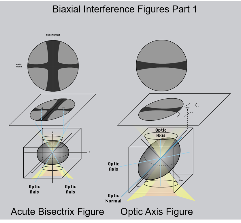
M= melatope; Bxa = acute bisectrix; Bxo = obtuse bisectrix.
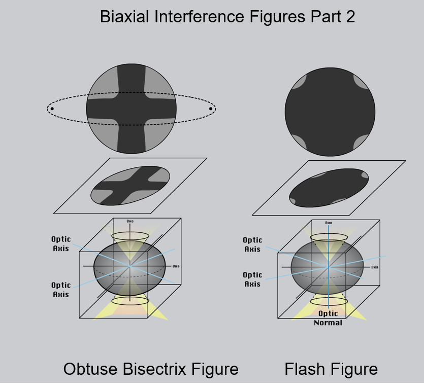
Bxa = acute bisectrix; Bxo = obtuse bisectrix.
Guided Inquiry
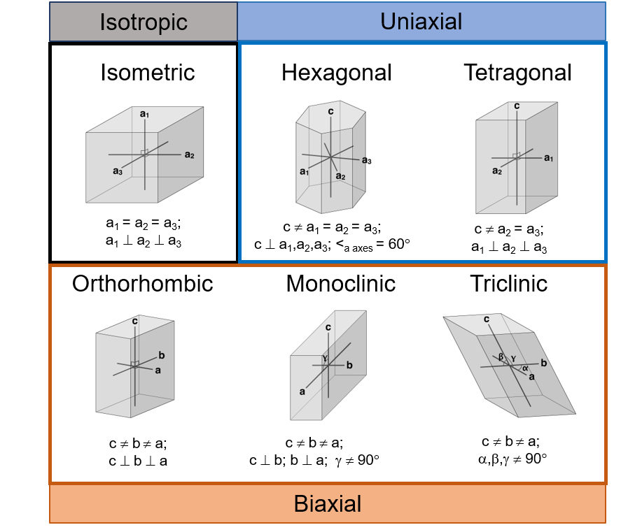
Interference Figures and Crystal Symmetry
The types of interference figures that a mineral produces are related to the crystal symmetry of that mineral. The figure below summarizes the division of crystal symmetries into isotropic, uniaxial, and biaxial optical properties.
Guided Inquiry
Synthesis: Is it Uniaxial or Biaxial?
Question \(\PageIndex{5}\)
Question \(\PageIndex{6}\)