2.7: Lab 7 - Fractures
- Page ID
- 12518
\( \newcommand{\vecs}[1]{\overset { \scriptstyle \rightharpoonup} {\mathbf{#1}} } \)
\( \newcommand{\vecd}[1]{\overset{-\!-\!\rightharpoonup}{\vphantom{a}\smash {#1}}} \)
\( \newcommand{\id}{\mathrm{id}}\) \( \newcommand{\Span}{\mathrm{span}}\)
( \newcommand{\kernel}{\mathrm{null}\,}\) \( \newcommand{\range}{\mathrm{range}\,}\)
\( \newcommand{\RealPart}{\mathrm{Re}}\) \( \newcommand{\ImaginaryPart}{\mathrm{Im}}\)
\( \newcommand{\Argument}{\mathrm{Arg}}\) \( \newcommand{\norm}[1]{\| #1 \|}\)
\( \newcommand{\inner}[2]{\langle #1, #2 \rangle}\)
\( \newcommand{\Span}{\mathrm{span}}\)
\( \newcommand{\id}{\mathrm{id}}\)
\( \newcommand{\Span}{\mathrm{span}}\)
\( \newcommand{\kernel}{\mathrm{null}\,}\)
\( \newcommand{\range}{\mathrm{range}\,}\)
\( \newcommand{\RealPart}{\mathrm{Re}}\)
\( \newcommand{\ImaginaryPart}{\mathrm{Im}}\)
\( \newcommand{\Argument}{\mathrm{Arg}}\)
\( \newcommand{\norm}[1]{\| #1 \|}\)
\( \newcommand{\inner}[2]{\langle #1, #2 \rangle}\)
\( \newcommand{\Span}{\mathrm{span}}\) \( \newcommand{\AA}{\unicode[.8,0]{x212B}}\)
\( \newcommand{\vectorA}[1]{\vec{#1}} % arrow\)
\( \newcommand{\vectorAt}[1]{\vec{\text{#1}}} % arrow\)
\( \newcommand{\vectorB}[1]{\overset { \scriptstyle \rightharpoonup} {\mathbf{#1}} } \)
\( \newcommand{\vectorC}[1]{\textbf{#1}} \)
\( \newcommand{\vectorD}[1]{\overrightarrow{#1}} \)
\( \newcommand{\vectorDt}[1]{\overrightarrow{\text{#1}}} \)
\( \newcommand{\vectE}[1]{\overset{-\!-\!\rightharpoonup}{\vphantom{a}\smash{\mathbf {#1}}}} \)
\( \newcommand{\vecs}[1]{\overset { \scriptstyle \rightharpoonup} {\mathbf{#1}} } \)
\( \newcommand{\vecd}[1]{\overset{-\!-\!\rightharpoonup}{\vphantom{a}\smash {#1}}} \)
\(\newcommand{\avec}{\mathbf a}\) \(\newcommand{\bvec}{\mathbf b}\) \(\newcommand{\cvec}{\mathbf c}\) \(\newcommand{\dvec}{\mathbf d}\) \(\newcommand{\dtil}{\widetilde{\mathbf d}}\) \(\newcommand{\evec}{\mathbf e}\) \(\newcommand{\fvec}{\mathbf f}\) \(\newcommand{\nvec}{\mathbf n}\) \(\newcommand{\pvec}{\mathbf p}\) \(\newcommand{\qvec}{\mathbf q}\) \(\newcommand{\svec}{\mathbf s}\) \(\newcommand{\tvec}{\mathbf t}\) \(\newcommand{\uvec}{\mathbf u}\) \(\newcommand{\vvec}{\mathbf v}\) \(\newcommand{\wvec}{\mathbf w}\) \(\newcommand{\xvec}{\mathbf x}\) \(\newcommand{\yvec}{\mathbf y}\) \(\newcommand{\zvec}{\mathbf z}\) \(\newcommand{\rvec}{\mathbf r}\) \(\newcommand{\mvec}{\mathbf m}\) \(\newcommand{\zerovec}{\mathbf 0}\) \(\newcommand{\onevec}{\mathbf 1}\) \(\newcommand{\real}{\mathbb R}\) \(\newcommand{\twovec}[2]{\left[\begin{array}{r}#1 \\ #2 \end{array}\right]}\) \(\newcommand{\ctwovec}[2]{\left[\begin{array}{c}#1 \\ #2 \end{array}\right]}\) \(\newcommand{\threevec}[3]{\left[\begin{array}{r}#1 \\ #2 \\ #3 \end{array}\right]}\) \(\newcommand{\cthreevec}[3]{\left[\begin{array}{c}#1 \\ #2 \\ #3 \end{array}\right]}\) \(\newcommand{\fourvec}[4]{\left[\begin{array}{r}#1 \\ #2 \\ #3 \\ #4 \end{array}\right]}\) \(\newcommand{\cfourvec}[4]{\left[\begin{array}{c}#1 \\ #2 \\ #3 \\ #4 \end{array}\right]}\) \(\newcommand{\fivevec}[5]{\left[\begin{array}{r}#1 \\ #2 \\ #3 \\ #4 \\ #5 \\ \end{array}\right]}\) \(\newcommand{\cfivevec}[5]{\left[\begin{array}{c}#1 \\ #2 \\ #3 \\ #4 \\ #5 \\ \end{array}\right]}\) \(\newcommand{\mattwo}[4]{\left[\begin{array}{rr}#1 \amp #2 \\ #3 \amp #4 \\ \end{array}\right]}\) \(\newcommand{\laspan}[1]{\text{Span}\{#1\}}\) \(\newcommand{\bcal}{\cal B}\) \(\newcommand{\ccal}{\cal C}\) \(\newcommand{\scal}{\cal S}\) \(\newcommand{\wcal}{\cal W}\) \(\newcommand{\ecal}{\cal E}\) \(\newcommand{\coords}[2]{\left\{#1\right\}_{#2}}\) \(\newcommand{\gray}[1]{\color{gray}{#1}}\) \(\newcommand{\lgray}[1]{\color{lightgray}{#1}}\) \(\newcommand{\rank}{\operatorname{rank}}\) \(\newcommand{\row}{\text{Row}}\) \(\newcommand{\col}{\text{Col}}\) \(\renewcommand{\row}{\text{Row}}\) \(\newcommand{\nul}{\text{Nul}}\) \(\newcommand{\var}{\text{Var}}\) \(\newcommand{\corr}{\text{corr}}\) \(\newcommand{\len}[1]{\left|#1\right|}\) \(\newcommand{\bbar}{\overline{\bvec}}\) \(\newcommand{\bhat}{\widehat{\bvec}}\) \(\newcommand{\bperp}{\bvec^\perp}\) \(\newcommand{\xhat}{\widehat{\xvec}}\) \(\newcommand{\vhat}{\widehat{\vvec}}\) \(\newcommand{\uhat}{\widehat{\uvec}}\) \(\newcommand{\what}{\widehat{\wvec}}\) \(\newcommand{\Sighat}{\widehat{\Sigma}}\) \(\newcommand{\lt}{<}\) \(\newcommand{\gt}{>}\) \(\newcommand{\amp}{&}\) \(\definecolor{fillinmathshade}{gray}{0.9}\)In this lab, you will meet two new techniques on the stereographic projection that are particularly useful for the analysis of joints and veins. Both involve small circles.
Orientation of veins from multiple boreholes
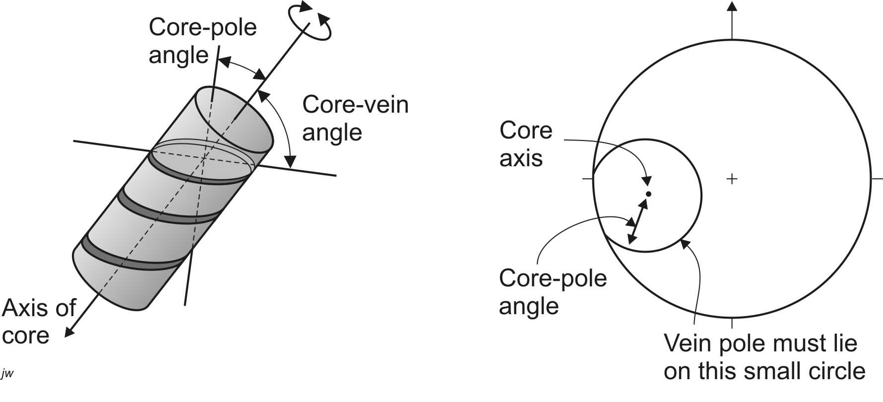
Many exploration programs are carried out to determine the location and orientation of buried mineralized veins. Typically, diamond-drill holes will be drilled at various angles into the ground and cores will be recovered, showing the orientation of the veins. Unfortunately, the drilling operation does not allow core to be recovered without rotating it in the drill hole, so a single core does not provide a unique indication of the strike and dip of a vein. All we can determine from a single core is that the pole to a vein must lie on a small circle on the stereographic projection (Fig. 1). It turns out that intersecting small circles from 3 cores are necessary to uniquely determine the orientaiton.
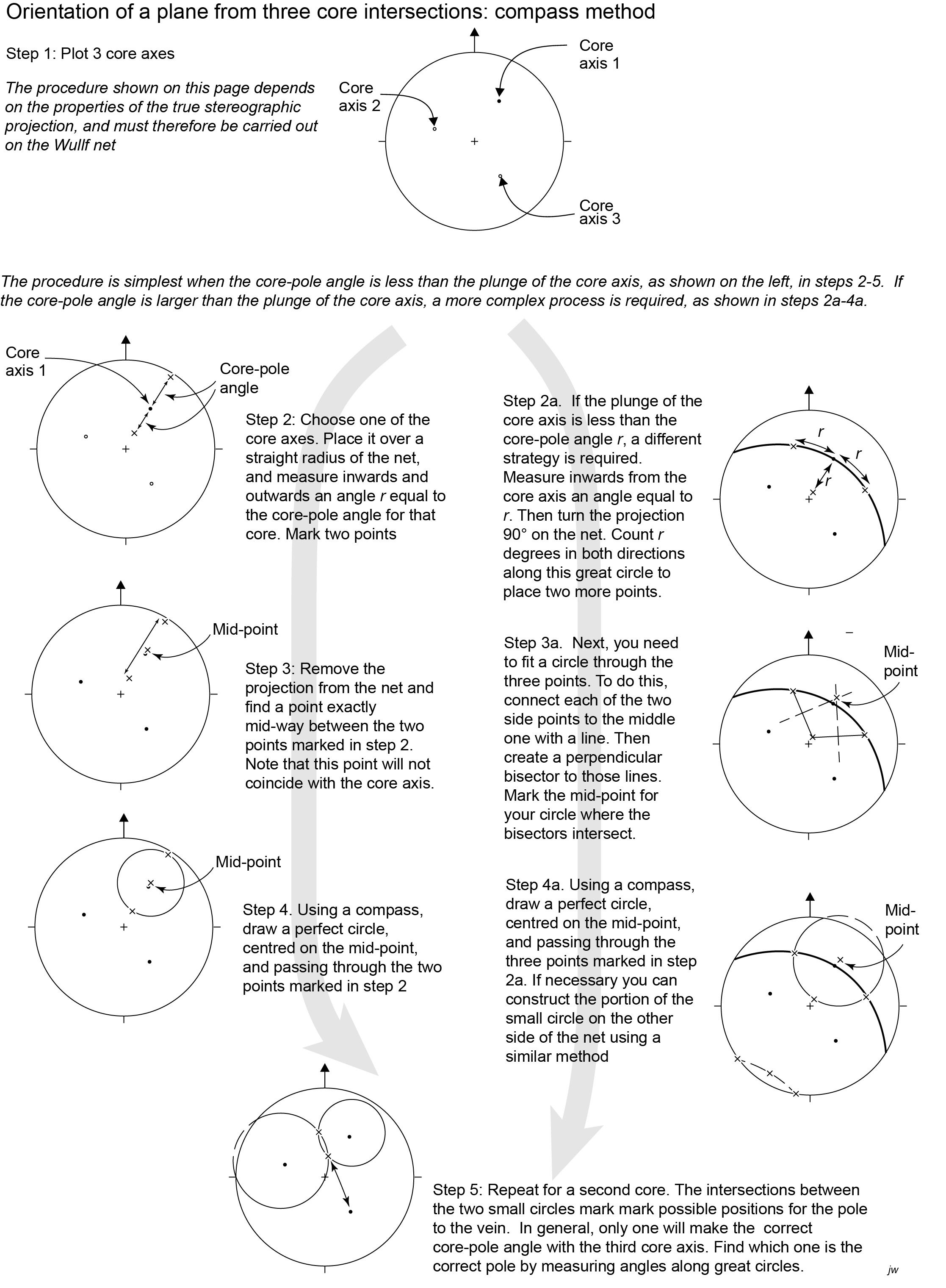
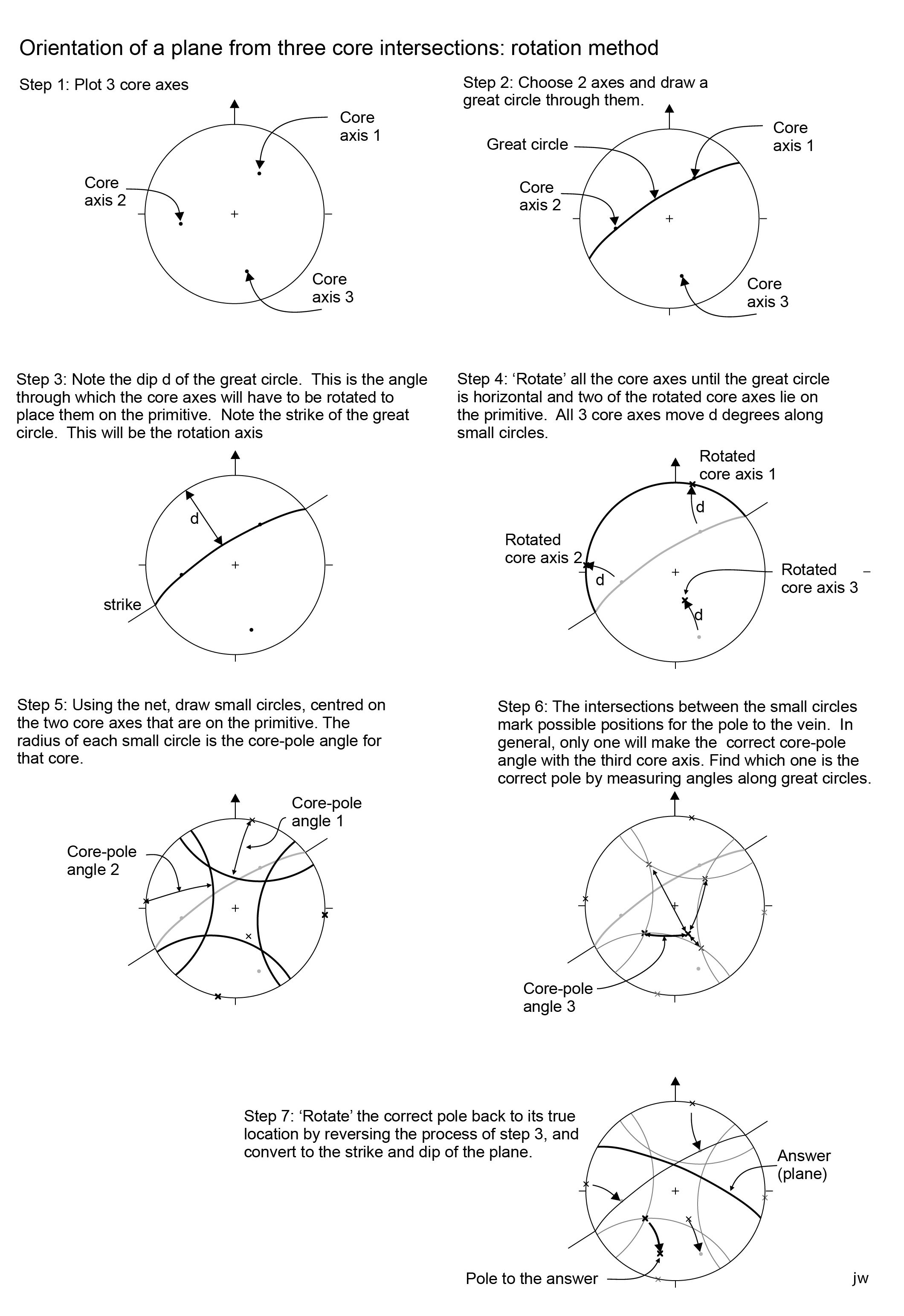
Constructing small circles can be complicated. If the cores are horizontal, it is easy, because the Wulff and Schmidt nets have small circles centred on the primitive. However, if the cores are plunging (the more usual case), constructing small circles is more involved. There are two methods. Method 1 depends on a property of the Wulff net, on which all small circles plot as true circles (as shown in Fig. 1) so it is possible to construct them with a plotting compass; however, the centre of the projected circle does not match the axis of the small circle in 3-D, so the centre of the point has to be found first. The process is simple if the small circles do not cross the primitive, but a little more involved if they do, as shown in Figure 2. Method 2 depends on rotating the orientations of the two cores to the primitive to construct the small circles there. Once the intersections are found, the rotation is reversed to find the true orientation of the intersections. The second procedure works on either the Wulff or Schmidt net and is explained in detail in Figure 3.
Density plots of poles
Sometimes large numbers of joints are measured in a particular area. Geologists may want to know the mean orientation of the joints, or to make statements about the variation in their orientation. Normal arithmetic methods for calculating averages don’t work for orientation data, because orientations are vector quantities. (To understand the problem, try finding the average of two trends close to north, 359° and 001°. The arithmetic average, 180° or due south, is obviously nonsense!)
It’s usually more helpful to start with a contoured plot showing the density of poles on a stereographic projection. Because we are analysing densities of poles, it is important to use an equal-area projection (Schmidt net) for this process.
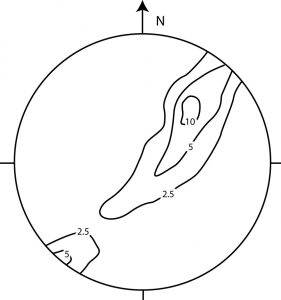
The first step in any contouring process is to superimpose the data on a grid. For this purpose you can either tape the projection down onto a piece of graph paper or you can draw a grid directly on the projection. For the example in the assignment, a grid has been drawn on a plot of poles.
Next, we need to find how many data points lie in each 1% of the net. To do this, a device called a counting circle is helpful. It can be a piece of paper with a circular hole, or a piece of tracing paper with a circle drawn on it.
In either case, the diameter of the circle must be exactly one tenth of the diameter of the equal-area net; its area will then be 1% of the net area.
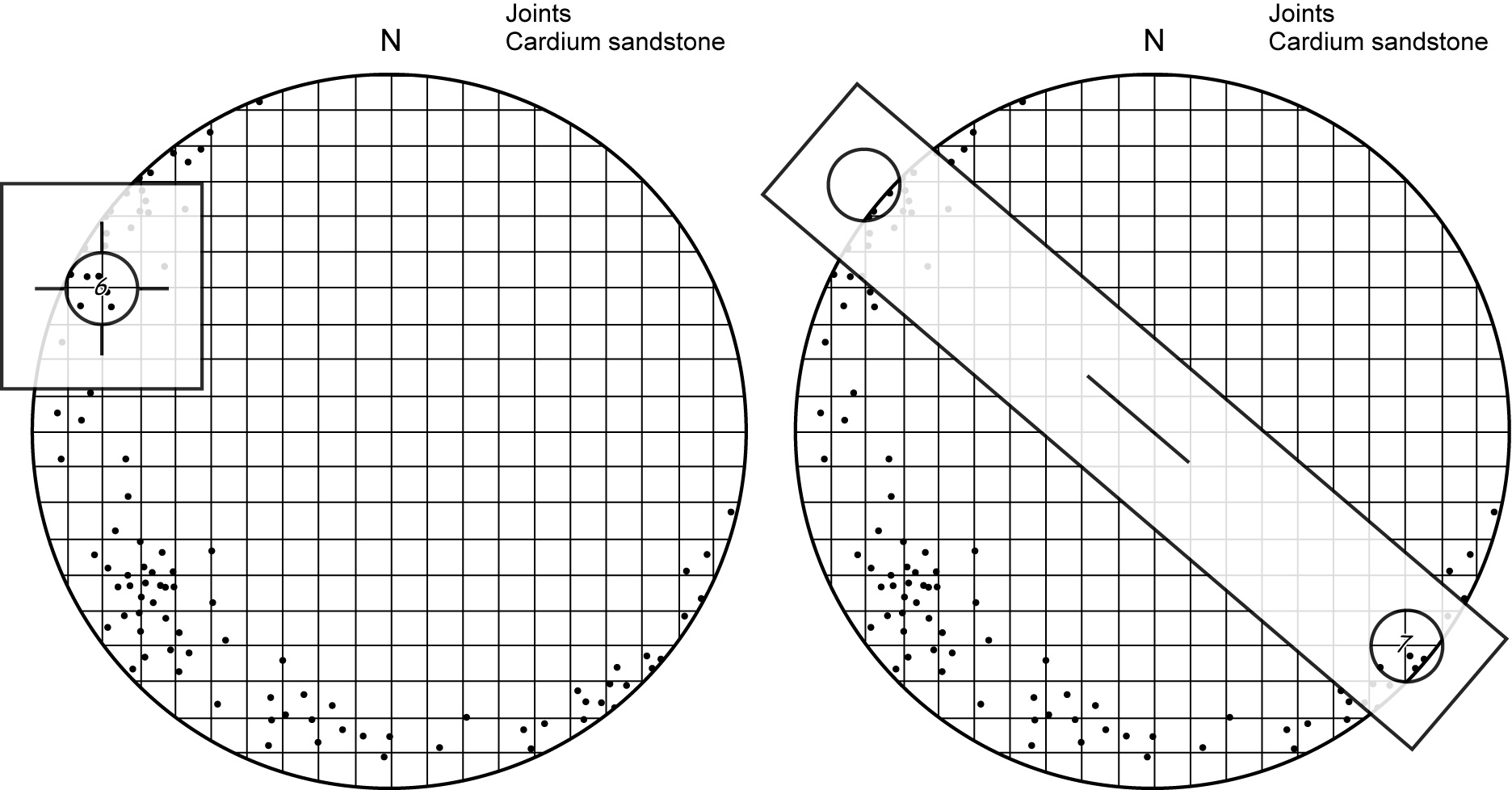
Place the counting circle directly over a grid intersection on the equal area plot. Count the number of poles that fall within the circle. Write this number on the grid intersection. Repeat with all the intersections in the plot.
For intersections that fall near the edge of the plot, part of the counting circle will fall outside the primitive. The points that ‘should’ be in this part of the counting circle will appear on the opposite side of the net. We therefore use a second device, called a peripheral counter, which has two counting circles, their centres spaced apart by the same distance as the diameter of the net. A slot in the centre of the peripheral counter fits over the thumb tack in the middle of the plot, so as to keep the counter correctly aligned. When one hole is centred over a grid intersection near the primitive, the circle on the opposite side contains the extra points that should be counted.
Finally, make a smooth contour map of the results. As in all contouring, make sure that higher numbers all appear on one side of a contour, and lower numbers on the other. Contours should never branch. In contouring, remember that contour lines that disappear over the primitive should reappear on the opposite side of the net. Number the contour lines in percent, meaning “percent of the data occurring in each 1 % of the plot area”.
Assignment
- A mineral exploration company drilled three diamond drill holes to intersect a vein set in the subsurface. The angles between the axes of the cores and the veins are shown in the following table.
| Drill hole # | Trend & plunge of hole | Core-vein angle | Core-pole angle |
| 1 | 340-70 NW | 40 | 50 |
| 2 | 080-76 NE | 65 | 25 |
| 3 | 210-68 SW | 54 | 36 |
Calculate the strike and dip of the vein set.
- You are provided with an equal area projection of 100 poles to conjugate shear fractures in the Cadomin Formation from the Alberta foothills. To find the maximum densities of points, it is helpful to construct a contoured plot. A grid has been constructed across the projection to assist with contouring.
a) First, cut out the centre counter and peripheral counting circles precisely. The counting circles have a diameter exactly 10% of the plot, which means that their area covers 1% of the plot. Use the counting circles to mark densities at the each grid intersection. Contour the resulting densities on the grid. Remember the principles of contouring that you used in the first lab: each contour should separate higher from lower values; make the contours as smooth as possible while honouring the data; contours should never branch. In addition, remember you are really contouring on the surface of a sphere, and the pattern is symmetrical on the lower and upper hemispheres. Therefore, if a contour disappears over the primitive, it should reappear on the opposite side of the projection. When you are done, make a clean copy with selected contours on a separate tracing sheet.
b) Mark estimated centres, or modes, of the two density clusters. These are poles to the typical conjugate shear planes. From these poles, determine the strike and dip of the two planes, and draw the planes as great circles on your plot.
The maximum principal stress is predicted to bisect the acute angle between the two planes. The minimum principal stress bisects the obtuse angle, and the intermediate stress is parallel to their intersection.
c) Mark the principal stresses on your contoured projection and determine the plunge and trend of each.
d) An oil company is interested in flow through extension joints in the Brazeau formation. Predict the orientation of these joints based on your estimates of the directions of the principal stresses.
Lab 7. Question 2. Plot of poles to 100 shear fractures in Cardium Sandstone, Alberta Foothills.
Lab 7. Question 2. Counting Tool
- *Look at the geological map of Canmore (east half) which shows numerous faults. Notice the band of dark blue Palliser Formation in the region north of Exshaw.
a) Without using the cross-section, what is the evidence that the Palliser Formation dips to the SW in this area?
b) Now look at the Palliser Formation on cross-section 1, which extends into the sheet Canmore (west half). Place two sheets of tracing paper so as to cover the cross-section, and trace only the base of the Palliser Formation (DPa) and the faults that offset it. For each of the named thrust faults, answer the following questions:
c) Does the fault place older over younger or younger over older strata?
d) Estimate the the dip separation of the base of the Palliser formation. Note – if the fault is curved, you can approximate the separation with a series of straight-line measurements with a ruler.
e) Estimate the throw and the heave. (These are straight line measurements even if the fault is curved.)
- *Strictly speaking, you have no evidence for the direction of movement on the faults: – it could be exactly parallel to the cross-section or there could be a component of strike-slip movement, in and out of the page. However, it is clear that there has been substantial overall shortening of the rocks in the hanging wall of the lowest, McConnell Thrust. Estimate this shortening in the line of the cross-section, as follows:
a) Measure the total original length l0 of the segments of the base of the Palliser Formation in the cross-section.
b) Measure the present-day distance l between the easternmost outcrop of the base of the Palliser, and the western edge of the section.
c) Calculate the shortening in kilometres: l0 – l.
d) Calculate the longitudinal strain as a value of stretch:s = l / l0.
e) Calculate the longitudinal strain as a fractional change in length or extension: e = (l – l0) / l
Map. Geology of Canmore (East Half)
Cross-sections. Geology of Canmore (East Half)


