2.6: Lab 6 - Fabrics and Folds
- Page ID
- 12515
\( \newcommand{\vecs}[1]{\overset { \scriptstyle \rightharpoonup} {\mathbf{#1}} } \)
\( \newcommand{\vecd}[1]{\overset{-\!-\!\rightharpoonup}{\vphantom{a}\smash {#1}}} \)
\( \newcommand{\id}{\mathrm{id}}\) \( \newcommand{\Span}{\mathrm{span}}\)
( \newcommand{\kernel}{\mathrm{null}\,}\) \( \newcommand{\range}{\mathrm{range}\,}\)
\( \newcommand{\RealPart}{\mathrm{Re}}\) \( \newcommand{\ImaginaryPart}{\mathrm{Im}}\)
\( \newcommand{\Argument}{\mathrm{Arg}}\) \( \newcommand{\norm}[1]{\| #1 \|}\)
\( \newcommand{\inner}[2]{\langle #1, #2 \rangle}\)
\( \newcommand{\Span}{\mathrm{span}}\)
\( \newcommand{\id}{\mathrm{id}}\)
\( \newcommand{\Span}{\mathrm{span}}\)
\( \newcommand{\kernel}{\mathrm{null}\,}\)
\( \newcommand{\range}{\mathrm{range}\,}\)
\( \newcommand{\RealPart}{\mathrm{Re}}\)
\( \newcommand{\ImaginaryPart}{\mathrm{Im}}\)
\( \newcommand{\Argument}{\mathrm{Arg}}\)
\( \newcommand{\norm}[1]{\| #1 \|}\)
\( \newcommand{\inner}[2]{\langle #1, #2 \rangle}\)
\( \newcommand{\Span}{\mathrm{span}}\) \( \newcommand{\AA}{\unicode[.8,0]{x212B}}\)
\( \newcommand{\vectorA}[1]{\vec{#1}} % arrow\)
\( \newcommand{\vectorAt}[1]{\vec{\text{#1}}} % arrow\)
\( \newcommand{\vectorB}[1]{\overset { \scriptstyle \rightharpoonup} {\mathbf{#1}} } \)
\( \newcommand{\vectorC}[1]{\textbf{#1}} \)
\( \newcommand{\vectorD}[1]{\overrightarrow{#1}} \)
\( \newcommand{\vectorDt}[1]{\overrightarrow{\text{#1}}} \)
\( \newcommand{\vectE}[1]{\overset{-\!-\!\rightharpoonup}{\vphantom{a}\smash{\mathbf {#1}}}} \)
\( \newcommand{\vecs}[1]{\overset { \scriptstyle \rightharpoonup} {\mathbf{#1}} } \)
\( \newcommand{\vecd}[1]{\overset{-\!-\!\rightharpoonup}{\vphantom{a}\smash {#1}}} \)
\(\newcommand{\avec}{\mathbf a}\) \(\newcommand{\bvec}{\mathbf b}\) \(\newcommand{\cvec}{\mathbf c}\) \(\newcommand{\dvec}{\mathbf d}\) \(\newcommand{\dtil}{\widetilde{\mathbf d}}\) \(\newcommand{\evec}{\mathbf e}\) \(\newcommand{\fvec}{\mathbf f}\) \(\newcommand{\nvec}{\mathbf n}\) \(\newcommand{\pvec}{\mathbf p}\) \(\newcommand{\qvec}{\mathbf q}\) \(\newcommand{\svec}{\mathbf s}\) \(\newcommand{\tvec}{\mathbf t}\) \(\newcommand{\uvec}{\mathbf u}\) \(\newcommand{\vvec}{\mathbf v}\) \(\newcommand{\wvec}{\mathbf w}\) \(\newcommand{\xvec}{\mathbf x}\) \(\newcommand{\yvec}{\mathbf y}\) \(\newcommand{\zvec}{\mathbf z}\) \(\newcommand{\rvec}{\mathbf r}\) \(\newcommand{\mvec}{\mathbf m}\) \(\newcommand{\zerovec}{\mathbf 0}\) \(\newcommand{\onevec}{\mathbf 1}\) \(\newcommand{\real}{\mathbb R}\) \(\newcommand{\twovec}[2]{\left[\begin{array}{r}#1 \\ #2 \end{array}\right]}\) \(\newcommand{\ctwovec}[2]{\left[\begin{array}{c}#1 \\ #2 \end{array}\right]}\) \(\newcommand{\threevec}[3]{\left[\begin{array}{r}#1 \\ #2 \\ #3 \end{array}\right]}\) \(\newcommand{\cthreevec}[3]{\left[\begin{array}{c}#1 \\ #2 \\ #3 \end{array}\right]}\) \(\newcommand{\fourvec}[4]{\left[\begin{array}{r}#1 \\ #2 \\ #3 \\ #4 \end{array}\right]}\) \(\newcommand{\cfourvec}[4]{\left[\begin{array}{c}#1 \\ #2 \\ #3 \\ #4 \end{array}\right]}\) \(\newcommand{\fivevec}[5]{\left[\begin{array}{r}#1 \\ #2 \\ #3 \\ #4 \\ #5 \\ \end{array}\right]}\) \(\newcommand{\cfivevec}[5]{\left[\begin{array}{c}#1 \\ #2 \\ #3 \\ #4 \\ #5 \\ \end{array}\right]}\) \(\newcommand{\mattwo}[4]{\left[\begin{array}{rr}#1 \amp #2 \\ #3 \amp #4 \\ \end{array}\right]}\) \(\newcommand{\laspan}[1]{\text{Span}\{#1\}}\) \(\newcommand{\bcal}{\cal B}\) \(\newcommand{\ccal}{\cal C}\) \(\newcommand{\scal}{\cal S}\) \(\newcommand{\wcal}{\cal W}\) \(\newcommand{\ecal}{\cal E}\) \(\newcommand{\coords}[2]{\left\{#1\right\}_{#2}}\) \(\newcommand{\gray}[1]{\color{gray}{#1}}\) \(\newcommand{\lgray}[1]{\color{lightgray}{#1}}\) \(\newcommand{\rank}{\operatorname{rank}}\) \(\newcommand{\row}{\text{Row}}\) \(\newcommand{\col}{\text{Col}}\) \(\renewcommand{\row}{\text{Row}}\) \(\newcommand{\nul}{\text{Nul}}\) \(\newcommand{\var}{\text{Var}}\) \(\newcommand{\corr}{\text{corr}}\) \(\newcommand{\len}[1]{\left|#1\right|}\) \(\newcommand{\bbar}{\overline{\bvec}}\) \(\newcommand{\bhat}{\widehat{\bvec}}\) \(\newcommand{\bperp}{\bvec^\perp}\) \(\newcommand{\xhat}{\widehat{\xvec}}\) \(\newcommand{\vhat}{\widehat{\vvec}}\) \(\newcommand{\uhat}{\widehat{\uvec}}\) \(\newcommand{\what}{\widehat{\wvec}}\) \(\newcommand{\Sighat}{\widehat{\Sigma}}\) \(\newcommand{\lt}{<}\) \(\newcommand{\gt}{>}\) \(\newcommand{\amp}{&}\) \(\definecolor{fillinmathshade}{gray}{0.9}\)Introduction
A fabric is essentially any structure that gives a rock different properties in one direction from another. In other words, some things in the rock have a preferred orientation. The ‘somethings’ in this case are the fabric elements. Although a fabric may be obvious, a close look may be necessary to determine what are the fabric elements.
Because fabrics and folds are both produced by strain, they commonly operate together. In the part of this lab that is map-based you are asked to unravel the structure of an area with both folds and fabrics.
Before you begin, make sure you are familiar with the earlier sections dealing with fold overprinting and with fabrics.
Note that the samples may only be available in the lab time.

Assignment.
1. *To illustrate the concept of fabric elements, you are provided with some everyday objects with simple fabric. For each fabric, determine:
-
- Is the fabric a foliation or a lineation?
- What are the fabric elements that define the fabric?
- What shape are the fabric elements (tabular, acicular, some combination)?
2. *Look at one rock sample from each group. Note that some of the samples have more than one fabric. For each sample, record the following:
-
- Identification of the sample;
- How many differently oriented planar fabrics (foliations)?
- How many differently oriented linear fabrics (lineations)?
For each fabric:
-
- Describe the elements that define the fabric;
- Does the fabric have a common name (slaty cleavage, crenulation lineation, etc.)?
- What is the relationship of the fabric to other fabrics in the rock? Where possible, number the fabrics S1, S2, L1, L2, etc….
3. You are provided a map of a group of glacially smoothed, low-lying islands showing metamorphic rock outcrops (Map 1). The structures are typically of the deeply eroded cores of many orogens. There are two generations of folds, with associated fabrics and asymmetric parasitic folds. A penetrative schistosity is present everywhere, together with a locally developed crenulation cleavage and crenulation lineation. In a few places, it is possible to see an intersection lineation between bedding and schistosity, though these two foliations are almost parallel in many outcrops, indicating that deformation has been intense.
a. Using an equal area projection, plot the orientations of the schistosity as poles.
b. Look at the folds on each island in turn. Notice that some of the folds deform the bedding but not the schistosity; these folds have axial planar schistosity, and therefore probably formed at around the same time as the schistosity. These folds are the first generation that can be identified in the area. Label them F1, in a distinctive colour (e.g. red). Other folds clearly formed after the schistosity because they fold the schistosity. Label these folds F2 in a contrasting colour (e.g. blue).
c. Label each F2 fold as S or Z based on its asymmetry. Use the same colour that you used to identify F2 folds.
d. Using your results from b and c, draw and label the principal fold axial trace for an F2 map-scale fold. Remember, a fold axial trace will separate S and Z senses of asymmetry. Label it using the F2 colour.
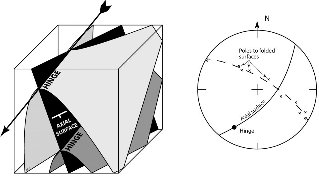
e. From your equal area projection, estimate the orientation of the F2 fold axis. Both the fold axis and the axial trace are lines that lie in the axial surface. Use these two lines to draw the axial surface as a great circle on your projection and determine its orientation. Add the crenulation cleavage and crenulation lineation to your projection. What is their relationship to the folds?
f. For each F1 fold, label it as S or Z based on its asymmetry, using the F1 colour. Draw the F1 axial traces on the map. (Remember, the F1 folds will probably have been refolded by F2, so you should not expect their traces to be straight!) Assuming the chlorite schist is the youngest unit, characterize the main F1 folds as either anticlines or synclines.
g. Add labels S0, S1, S2, L1, etc. to the legend where indicated by ‘…..’
h. Complete the map as far as possible in the unexposed areas between the islands to show the overall structure (to help you visualize the structure, you may wish to sketch a cross-section AB, but this is not required).


